4 Query Optimizer Concepts
This chapter describes the most important concepts relating to the query optimizer. This chapter contains the following topics:
4.1 Introduction to the Query Optimizer
The query optimizer (called simply the optimizer) is built-in database software that determines the most efficient method for a SQL statement to access requested data.
This section contains the following topics:
4.1.1 Purpose of the Query Optimizer
The optimizer attempts to generate the best execution plan for a SQL statement. The best execution plan is defined as the plan with the lowest cost among all considered candidate plans. The cost computation accounts for factors of query execution such as I/O, CPU, and communication.
The best method of execution depends on myriad conditions including how the query is written, the size of the data set, the layout of the data, and which access structures exist. The optimizer determines the best plan for a SQL statement by examining multiple access methods, such as full table scan or index scans, and different join methods such as nested loops and hash joins.
Because the database has many internal statistics and tools at its disposal, the optimizer is usually in a better position than the user to determine the best method of statement execution. For this reason, all SQL statements use the optimizer.
Consider a user who queries records for employees who are managers. If the database statistics indicate that 80% of employees are managers, then the optimizer may decide that a full table scan is most efficient. However, if statistics indicate that few employees are managers, then reading an index followed by a table access by rowid may be more efficient than a full table scan.
4.1.2 Cost-Based Optimization
Query optimization is the overall process of choosing the most efficient means of executing a SQL statement. SQL is a nonprocedural language, so the optimizer is free to merge, reorganize, and process in any order.
The database optimizes each SQL statement based on statistics collected about the accessed data. When generating execution plans, the optimizer considers different access paths and join methods. Factors considered by the optimizer include:
-
System resources, which includes I/O, CPU, and memory
-
Number of rows returned
-
Size of the initial data sets
The cost is a number that represents the estimated resource usage for an execution plan. The optimizer assigns a cost to each possible plan, and then chooses the plan with the lowest cost. For this reason, the optimizer is sometimes called the cost-based optimizer (CBO) to contrast it with the legacy rule-based optimizer (RBO).
Note:
The optimizer may not make the same decisions from one version of Oracle Database to the next. In recent versions, the optimizer might make different decision because better information is available and more optimizer transformations are possible.4.1.3 Execution Plans
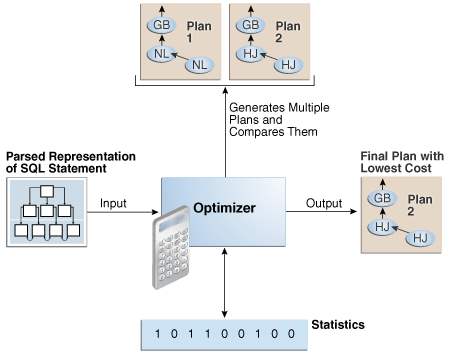
An execution plan describes a recommended method of execution for a SQL statement. The plans shows the combination of the steps Oracle Database uses to execute a SQL statement. Each step either retrieves rows of data physically from the database or prepares them for the user issuing the statement.
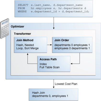
In Figure 4-1, the optimizer generates two possible execution plans for an input SQL statement, uses statistics to calculate their costs, compares their costs, and chooses the plan with the lowest cost.
4.1.3.1 Query Blocks
As shown in Figure 4-1, the input to the optimizer is a parsed representation of a SQL statement. Each SELECT block in the original SQL statement is represented internally by a query block. A query block can be a top-level statement, subquery, or unmerged view (see "View Merging").
In Example 4-1, the SQL statement consists of two query blocks. The subquery in parentheses is the inner query block. The outer query block, which is the rest of the SQL statement, retrieves names of employees in the departments whose IDs were supplied by the subquery.
SELECT first_name, last_name
FROM   hr.employees
WHERE  department_id
IN     (SELECT department_id
        FROM   hr.departments
        WHERE  location_id = 1800);
The query form determines how query blocks are interrelated.
See Also:
Oracle Database Concepts for an overview of SQL processing4.1.3.2 Query Subplans
For each query block, the optimizer generates a query subplan. The database optimizes query blocks separately from the bottom up. Thus, the database optimizes the innermost query block first and generates a subplan for it, and then generates the outer query block representing the entire query.
The number of possible plans for a query block is proportional to the number of objects in the FROM clause. This number rises exponentially with the number of objects. For example, the possible plans for a join of five tables are significantly higher than the possible plans for a join of two tables.
4.1.3.3 Analogy for the Optimizer
One analogy for the optimizer is an online trip advisor. A cyclist wants to know the most efficient bicycle route from point A to point B. A query is like the directive "I need the most efficient route from point A to point B" or "I need the most efficient route from point A to point B by way of point C." The trip advisor uses an internal algorithm, which relies on factors such as speed and difficulty, to determine the most efficient route. The cyclist can influence the trip advisor's decision by using directives such as "I want to arrive as fast as possible" or "I want the easiest ride possible."
In this analogy, an execution plan is a possible route generated by the trip advisor. Internally, the advisor may divide the overall route into several subroutes (subplans), and calculate the efficiency for each subroute separately. For example, the trip advisor may estimate one subroute at 15 minutes with medium difficulty, an alternative subroute at 22 minutes with minimal difficulty, and so on.
The advisor picks the most efficient (lowest cost) overall route based on user-specified goals and the available statistics about roads and traffic conditions. The more accurate the statistics, the better the advice. For example, if the advisor is not frequently notified of traffic jams, road closures, and poor road conditions, then the recommended route may turn out to be inefficient (high cost).
4.2 About Optimizer Components
The optimizer contains three main components, which are shown in Figure 4-2.
A set of query blocks represents a parsed query, which is the input to the optimizer. The optimizer performs the following operations:
-
Query transformer
The optimizer determines whether it is helpful to change the form of the query so that the optimizer can generate a better execution plan. See "Query Transformer".
-
Estimator
The optimizer estimates the cost of each plan based on statistics in the data dictionary. See "Estimator".
-
Plan Generator
The optimizer compares the costs of plans and chooses the lowest-cost plan, known as the execution plan, to pass to the row source generator. See "Plan Generator".
4.2.1 Query Transformer
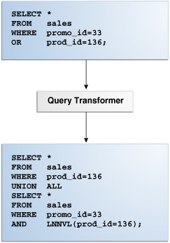
For some statements, the query transformer determines whether it is advantageous to rewrite the original SQL statement into a semantically equivalent SQL statement with a lower cost. When a viable alternative exists, the database calculates the cost of the alternatives separately and chooses the lowest-cost alternative. Chapter 5, "Query Transformations" describes the different types of optimizer transformations.
Figure 4-3 shows the query transformer rewriting an input query that uses OR into an output query that uses UNION ALL.
See Also:
Chapter 5, "Query Transformations"4.2.2 Estimator
The estimator is the component of the optimizer that determines the overall cost of a given execution plan. The estimator uses three different types of measures to achieve this goal:
-
The percentage of rows in the row set that the query selects, with
0meaning no rows and1meaning all rows. Selectivity is tied to a query predicate, such asWHERE last_name LIKE 'A%', or a combination of predicates. A predicate becomes more selective as the selectivity value approaches0and less selective (or more unselective) as the value approaches1.Note:
Selectivity is an internal calculation that is not visible in the execution plans. -
The cardinality is the estimated number of rows returned by each operation in an execution plan. This input, which is crucial to obtaining an optimal plan, is common to all cost functions. Cardinality can be derived from the table statistics collected by
DBMS_STATS, or derived after accounting for effects from predicates (filter, join, and so on),DISTINCTorGROUP BYoperations, and so on. -
This measure represents units of work or resource used. The query optimizer uses disk I/O, CPU usage, and memory usage as units of work.
As shown in Figure 4-4, if statistics are available, then the estimator uses them to compute the measures. The statistics improve the degree of accuracy of the measures.
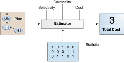
For the query shown in Example 4-1, the estimator uses selectivity, cardinality, and cost measures to produce its total cost estimate of 3:
----------------------------------------------------------------------------------
| Id| Operation                    |Name             |Rows|Bytes|Cost(%CPU)| Time|
----------------------------------------------------------------------------------
| 0 | SELECT STATEMENT             |                 |  10|  250| 3 (0)| 00:00:01|
| 1 |  NESTED LOOPS                |                 |    |     |      |         |
| 2 |   NESTED LOOPS               |                 |  10|  250| 3 (0)| 00:00:01|
|*3 |    TABLE ACCESS FULL         |DEPARTMENTS      |   1|    7| 2 (0)| 00:00:01|
|*4 |    INDEX RANGE SCAN          |EMP_DEPARTMENT_IX|  10|     | 0 (0)| 00:00:01|
| 5 |   TABLE ACCESS BY INDEX ROWID|EMPLOYEES        |  10|  180| 1 (0)| 00:00:01|
----------------------------------------------------------------------------------
4.2.2.1 Selectivity
The selectivity represents a fraction of rows from a row set. The row set can be a base table, a view, or the result of a join. The selectivity is tied to a query predicate, such as last_name = 'Smith', or a combination of predicates, such as last_name = 'Smith' AND job_id = 'SH_CLERK'.
Note:
Selectivity is an internal calculation that is not visible in execution plans.A predicate filters a specific number of rows from a row set. Thus, the selectivity of a predicate indicates how many rows pass the predicate test. Selectivity ranges from 0.0 to 1.0. A selectivity of 0.0 means that no rows are selected from a row set, whereas a selectivity of 1.0 means that all rows are selected. A predicate becomes more selective as the value approaches 0.0 and less selective (or more unselective) as the value approaches 1.0.
The optimizer estimates selectivity depending on whether statistics are available:
-
Statistics not available
Depending on the value of the
OPTIMIZER_DYNAMIC_SAMPLINGinitialization parameter, the optimizer either uses dynamic statistics or an internal default value. The database uses different internal defaults depending on the predicate type. For example, the internal default for an equality predicate (last_name='Smith') is lower than for a range predicate (last_name >'Smith') because an equality predicate is expected to return a smaller fraction of rows. -
Statistics available
When statistics are available, the estimator uses them to estimate selectivity. Assume there are 150 distinct employee last names. For an equality predicate
last_name ='Smith', selectivity is the reciprocal of the numbernof distinct values oflast_name, which in this example is .006 because the query selects rows that contain 1 out of 150 distinct values.If a histogram exists on the
last_namecolumn, then the estimator uses the histogram instead of the number of distinct values. The histogram captures the distribution of different values in a column, so it yields better selectivity estimates, especially for columns that have data skew. See Chapter 11, "Histograms."
4.2.2.2 Cardinality
The cardinality is the estimated number of rows returned by each operation in an execution plan. For example, if the optimizer estimate for the number of rows returned by a full table scan is 100, then the cardinality for this operation is 100. The cardinality value appears in the Rows column of the execution plan.
The optimizer determines the cardinality for each operation based on a complex set of formulas that use both table and column level statistics, or dynamic statistics, as input. The optimizer uses one of the simplest formulas when a single equality predicate appears in a single-table query, with no histogram. In this case, the optimizer assumes a uniform distribution and calculates the cardinality for the query by dividing the total number of rows in the table by the number of distinct values in the column used in the WHERE clause predicate.
For example, user hr queries the employees table as follows:
SELECT first_name, last_name
FROM   employees
WHERE  salary='10200';
The employees table contains 107 rows. The current database statistics indicate that the number of distinct values in the salary column is 58. Thus, the optimizer calculates the cardinality of the result set as 2, using the formula 107/58=1.84.
Cardinality estimates must be as accurate as possible because they influence all aspects of the execution plan. Cardinality is important when the optimizer determines the cost of a join. For example, in a nested loops join of the employees and departments tables, the number of rows in employees determines how often the database must probe the departments table. Cardinality is also important for determining the cost of sorts.
4.2.2.3 Cost
The optimizer cost model accounts for the I/O, CPU, and network resources that a query is predicted to use. The cost is an internal numeric measure that represents the estimated resource usage for a plan. The lower the cost, the more efficient the plan.
The execution plan displays the cost of the entire plan, which is indicated on line 0, and each individual operation. For example, the following plan shows a cost of 14.
EXPLAINED SQL STATEMENT:
------------------------
SELECT prod_category, AVG(amount_sold) FROM   sales s, products p WHERE
 p.prod_id = s.prod_id GROUP BY prod_category

Plan hash value: 4073170114

----------------------------------------------------------------------
| Id  | Operation                | Name                 | Cost (%CPU)|
----------------------------------------------------------------------
|   0 | SELECT STATEMENT         |                      |    14 (100)|
|   1 |  HASH GROUP BY           |                      |    14  (22)|
|   2 |   HASH JOIN              |                      |    13  (16)|
|   3 |    VIEW                  | index$_join$_002     |     7  (15)|
|   4 |     HASH JOIN            |                      |            |
|   5 |      INDEX FAST FULL SCAN| PRODUCTS_PK          |     4   (0)|
|   6 |      INDEX FAST FULL SCAN| PRODUCTS_PROD_CAT_IX |     4   (0)|
|   7 |    PARTITION RANGE ALL   |                      |     5   (0)|
|   8 |     TABLE ACCESS FULL    | SALES                |     5   (0)|
----------------------------------------------------------------------
The cost is an internal unit that you can use for plan comparisons. You cannot tune or change it.
The access path determines the number of units of work required to get data from a base table. The access path can be a table scan, a fast full index scan, or an index scan.
-
Table scan or fast full index scan
During a table scan or fast full index scan, the database reads multiple blocks from disk in a single I/O. Therefore, the cost of the scan depends on the number of blocks to be scanned and the multiblock read count value.
-
Index scan
The cost of an index scan depends on the levels in the B-tree, the number of index leaf blocks to be scanned, and the number of rows to be fetched using the rowid in the index keys. The cost of fetching rows using rowids depends on the index clustering factor.
The join cost represents the combination of the individual access costs of the two row sets being joined, plus the cost of the join operation.
4.2.3 Plan Generator
The plan generator explores various plans for a query block by trying out different access paths, join methods, and join orders. Many plans are possible because of the various combinations that the database can use to produce the same result. The optimizer picks the plan with the lowest cost.
Figure 4-5 shows the optimizer testing different plans for an input query.
The following snippet from an optimizer trace file shows some computations that the optimizer performs:
GENERAL PLANS
***************************************
Considering cardinality-based initial join order.
Permutations for Starting Table :0
Join order[1]:  DEPARTMENTS[D]#0  EMPLOYEES[E]#1

***************
Now joining: EMPLOYEES[E]#1
***************
NL Join
  Outer table: Card: 27.00  Cost: 2.01  Resp: 2.01  Degree: 1  Bytes: 16
Access path analysis for EMPLOYEES
. . .
  Best NL cost: 13.17
. . .
SM Join
  SM cost: 6.08
     resc: 6.08 resc_io: 4.00 resc_cpu: 2501688
     resp: 6.08 resp_io: 4.00 resp_cpu: 2501688
. . .
SM Join (with index on outer)
  Access Path: index (FullScan)
. . .
HA Join
  HA cost: 4.57
     resc: 4.57 resc_io: 4.00 resc_cpu: 678154
     resp: 4.57 resp_io: 4.00 resp_cpu: 678154
Best:: JoinMethod: Hash
       Cost: 4.57  Degree: 1  Resp: 4.57  Card: 106.00 Bytes: 27
. . .

***********************
Join order[2]:  EMPLOYEES[E]#1  DEPARTMENTS[D]#0
. . .

***************
Now joining: DEPARTMENTS[D]#0
***************
. . .
HA Join
  HA cost: 4.58
     resc: 4.58 resc_io: 4.00 resc_cpu: 690054
     resp: 4.58 resp_io: 4.00 resp_cpu: 690054
Join order aborted: cost > best plan cost
***********************
The trace file shows the optimizer first trying the departments table as the outer table in the join. The optimizer calculates the cost for three different join methods: nested loops join (NL), sort merge (SM), and hash join (HA). The optimizer picks the hash join as the most efficient method:
Best:: JoinMethod: Hash
       Cost: 4.57  Degree: 1  Resp: 4.57  Card: 106.00 Bytes: 27
The optimizer then tries a different join order, using employees as the outer table. This join order costs more than the previous join order, so it is abandoned.
The optimizer uses an internal cutoff to reduce the number of plans it tries when finding the lowest-cost plan. The cutoff is based on the cost of the current best plan. If the current best cost is large, then the optimizer explores alternative plans to find a lower cost plan. If the current best cost is small, then the optimizer ends the search swiftly because further cost improvement is not significant.
4.3 About Automatic Tuning Optimizer
The optimizer performs different operations depending on how it is invoked. The database provides the following types of optimization:
-
Normal optimization
The optimizer compiles the SQL and generates an execution plan. The normal mode generates a reasonable plan for most SQL statements. Under normal mode, the optimizer operates with strict time constraints, usually a fraction of a second, during which it must find an optimal plan.
-
SQL Tuning Advisor optimization
When SQL Tuning Advisor invokes the optimizer, the optimizer is known as Automatic Tuning Optimizer. In this case, the optimizer performs additional analysis to further improve the plan produced in normal mode. The optimizer output is not an execution plan, but a series of actions, along with their rationale and expected benefit for producing a significantly better plan.
4.4 About Adaptive Query Optimization
In Oracle Database, adaptive query optimization is a set of capabilities that enables the optimizer to make run-time adjustments to execution plans and discover additional information that can lead to better statistics. Adaptive optimization is helpful when existing statistics are not sufficient to generate an optimal plan.
The following graphic shows the feature set for adaptive query optimization:
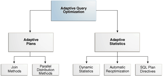
Description of the illustration tgsql_vm_069.png
4.4.1 Adaptive Plans
An adaptive plan enables the optimizer to defer the final plan decision for a statement until execution time. The ability of the optimizer to adapt a plan, based on information learned during execution, can greatly improve query performance.
Adaptive plans are useful because the optimizer occasionally picks a suboptimal default plan because of a cardinality misestimate. The ability to adapt the plan at run time based on actual execution statistics results in a more optimal final plan. After choosing the final plan, the optimizer uses it for subsequent executions, thus ensuring that the suboptimal plan is not reused.
See Also:
4.4.1.1 How Adaptive Plans Work
An adaptive plan contains multiple predetermined subplans, and an optimizer statistics collector. A subplan is a portion of a plan that the optimizer can switch to as an alternative at run time. For example, a nested loops join could be switched to a hash join during execution. An optimizer statistics collector is a row source inserted into a plan at key points to collect run-time statistics. These statistics help the optimizer make a final decision between multiple subplans.
During statement execution, the statistics collector gathers information about the execution, and buffers some rows received by the subplan. Based on the information observed by the collector, the optimizer chooses a subplan. At this point, the collector stops collecting statistics and buffering rows, and permits rows to pass through instead. On subsequent executions of the child cursor, the optimizer continues to use the same plan unless the plan ages out of the cache, or a different optimizer feature (for example, adaptive cursor sharing or statistics feedback) invalidates the plan.
The database uses adaptive plans when OPTIMIZER_FEATURES_ENABLE is 12.1.0.1 or later, and the OPTIMIZER_ADAPTIVE_REPORTING_ONLY initialization parameter is set to the default of false (see "Controlling Adaptive Optimization").
4.4.1.2 Adaptive Plans: Join Method Example
Example 4-2 shows a join of the order_items and product_information tables. An adaptive plan for this statement shows two possible plans, one with a nested loops join and the other with a hash join.
Example 4-2 Join of order_items and product_information
SELECT product_name
FROM   order_items o, product_information p
WHERE  o.unit_price = 15
AND    quantity > 1
AND    p.product_id = o.product_id
A nested loops join is preferable if the database can avoid scanning a significant portion of product_information because its rows are filtered by the join predicate. If few rows are filtered, however, then scanning the right table in a hash join is preferable.
The following graphic shows the adaptive process. For the query in Example 4-2, the adaptive portion of the default plan contains two subplans, each of which uses a different join method. The optimizer automatically determines when each join method is optimal, depending on the cardinality of the left side of the join.
The statistics collector buffers enough rows coming from the order_items table to determine which join method to use. If the row count is below the threshold determined by the optimizer, then the optimizer chooses the nested loops join; otherwise, the optimizer chooses the hash join. In this case, the row count coming from the order_items table is above the threshold, so the optimizer chooses a hash join for the final plan, and disables buffering.
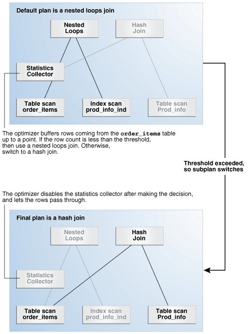
Description of the illustration tgsql_vm_076.png
After the optimizer determines the final plan, DBMS_XPLAN.DISPLAY_CURSOR displays the hash join. The Note section of the execution plan indicates whether the plan is adaptive, as shown in the following sample plan:
----------------------------------------------------------------------------------------------------------------
|Id | Operation          | Name                |Starts|E-Rows|A-Rows|   A-Time   |Buffers|Reads|OMem|1Mem|O/1/M|
----------------------------------------------------------------------------------------------------------------
|  0| SELECT STATEMENT   |                     | 1 |   |  13 |00:00:00.10 |  21 |  17 |       |       |        |
|* 1|  HASH JOIN         |                     | 1 | 4 |  13 |00:00:00.10 |  21 |  17 |  2061K|  2061K|   1/0/0|
|* 2|   TABLE ACCESS FULL| ORDER_ITEMS         | 1 | 4 |  13 |00:00:00.07 |   5 |   4 |       |       |        |
|  3|   TABLE ACCESS FULL| PRODUCT_INFORMATION | 1 | 1 | 288 |00:00:00.03 |  16 |  13 |       |       |        |
----------------------------------------------------------------------------------------------------------------

Predicate Information (identified by operation id):
---------------------------------------------------

   1 - access("P"."PRODUCT_ID"="O"."PRODUCT_ID")
   2 - filter(("O"."UNIT_PRICE"=15 AND "QUANTITY">1))


PLAN_TABLE_OUTPUT
----------------------------------------------------------------------------------------------------------------
Note
-----
   - this is an adaptive plan
See Also:
-
"Reading Execution Plans: Advanced" for an extended example showing an adaptive plan
4.4.1.3 Adaptive Plans: Parallel Distribution Methods
Typically, parallel execution requires data redistribution to perform operations such as parallel sorts, aggregations, and joins. Oracle Database can use many different data distributions methods. The database chooses the method based on the number of rows to be distributed and the number of parallel server processes in the operation.
For example, consider the following alternative cases:
-
Many parallel server processes distribute few rows.
The database may choose the broadcast distribution method. In this case, each row in the result set is sent to each of the parallel server processes.
-
Few parallel server processes distribute many rows.
If a data skew is encountered during the data redistribution, then it could adversely effect the performance of the statement. The database is more likely to pick a hash distribution to ensure that each parallel server process receives an equal number of rows.
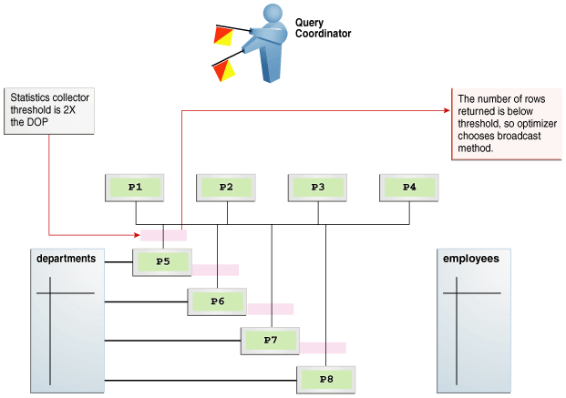
The hybrid hash distribution technique is an adaptive parallel data distribution that does not decide the final data distribution method until execution time. The optimizer inserts statistic collectors in front of the parallel server processes on the producer side of the operation. If the actual number of rows is less than a threshold, defined as twice the degree of parallelism (DOP) chosen for the operation, then the data distribution method switches from hash to broadcast. Otherwise, the distribution method is a hash.
Figure 4-6 depicts a hybrid hash join between the departments and employees tables, with a query coordinator directing 8 PX server processes. A statistics collector is inserted in front of the parallel server processes scanning the departments table. The distribution method is based on the run-time statistics. In the example shown in Figure 4-6, the number of rows is below the threshold (8), which is twice the DOP (4), so the optimizer chooses a broadcast technique for the departments table.
Contrast the broadcast distribution example in Figure 4-6 with an example that returns a greater number of rows. In the following plan, the threshold is 8, or twice the specified DOP of 4. However, because the statistics collector (Step 10) discovers that the number of rows (27) is greater than the threshold (8), the optimizer chooses a hybrid hash distribution rather than a broadcast distribution.
EXPLAIN PLAN FOR
  SELECT /*+ parallel(4) full(e) full(d) */ department_name, sum(salary)
  FROM   employees e, departments d
  WHERE  d.department_id=e.department_id
  GROUP BY department_name;

Plan hash value: 2940813933
----------------------------------------------------------------------------------------------------------------
| Id| Operation                          | Name      | Rows|Bytes|Cost   |Time      |    TQ |IN-OUT|PQ Distrib |
----------------------------------------------------------------------------------------------------------------
|  0| SELECT STATEMENT                   |DEPARTMENTS|  27 | 621 | 6 (34)| 00:00:01 |       |      |           |
|  1|  PX COORDINATOR                    |           |     |     |       |          |       |      |           |
|  2|   PX SEND QC (RANDOM)              | :TQ10003  |  27 | 621 | 6 (34)| 00:00:01 | Q1,03 | P->S | QC (RAND) |
|  3|    HASH GROUP BY                   |           |  27 | 621 | 6 (34)| 00:00:01 | Q1,03 | PCWP |           |
|  4|     PX RECEIVE                     |           |  27 | 621 | 6 (34)| 00:00:01 | Q1,03 | PCWP |           |
|  5|      PX SEND HASH                  | :TQ10002  |  27 | 621 | 6 (34)| 00:00:01 | Q1,02 | P->P | HASH      |
|  6|       HASH GROUP BY                |           |  27 | 621 | 6 (34)| 00:00:01 | Q1,02 | PCWP |           |
|* 7|        HASH JOIN                   |           | 106 |2438 | 5 (20)| 00:00:01 | Q1,02 | PCWP |           |
|  8|         PX RECEIVE                 |           |  27 | 432 | 2  (0)| 00:00:01 | Q1,02 | PCWP |           |
|  9|          PX SEND HYBRID HASH       | :TQ10000  |  27 | 432 | 2  (0)| 00:00:01 | Q1,00 | P->P |HYBRID HASH|
| 10|           STATISTICS COLLECTOR     |           |     |     |       |          | Q1,00 | PCWC |           |
| 11|            PX BLOCK ITERATOR       |           |  27 | 432 | 2  (0)| 00:00:01 | Q1,00 | PCWC |           |
| 12|             TABLE ACCESS FULL      |DEPARTMENTS|  27 | 432 | 2  (0)| 00:00:01 | Q1,00 | PCWP |           |
| 13|         PX RECEIVE                 |           | 107 | 749 | 2  (0)| 00:00:01 | Q1,02 | PCWP |           |
| 14|          PX SEND HYBRID HASH (SKEW)| :TQ10001  | 107 | 749 | 2  (0)| 00:00:01 | Q1,01 | P->P |HYBRID HASH|
| 15|           PX BLOCK ITERATOR        |           | 107 | 749 | 2  (0)| 00:00:01 | Q1,01 | PCWC |           |
| 16|            TABLE ACCESS FULL       |EMPLOYEES  | 107 | 749 | 2  (0)| 00:00:01 | Q1,01 | PCWP |           |
----------------------------------------------------------------------------------------------------------------

Predicate Information (identified by operation id):---------------------------------------------------

   7 - access("D"."DEPARTMENT_ID"="E"."DEPARTMENT_ID")

Note
-----
   - Degree of Parallelism is 4 because of hint

32 rows selected.
See Also:
Oracle Database VLDB and Partitioning Guide to learn more about parallel data redistribution techniques4.4.2 Adaptive Statistics
The quality of the plans that the optimizer generates depends on the quality of the statistics. Some query predicates become too complex to rely on base table statistics alone, so the optimizer augments these statistics with adaptive statistics.
The following topics describe types of adaptive statistics:
4.4.2.1 Dynamic Statistics
During the compilation of a SQL statement, the optimizer decides whether to use dynamic statistics by considering whether the available statistics are sufficient to generate an optimal execution plan. If the available statistics are insufficient, then the optimizer uses dynamic statistics to augment the statistics. One type of dynamic statistics is the information gathered by dynamic sampling. The optimizer can use dynamic statistics for table scans, index access, joins, and GROUP BY operations, thus improving the quality of optimizer decisions.
See Also:
"Dynamic Statistics" to learn more about dynamic statistics and optimizer statistics in general4.4.2.2 Automatic Reoptimization
Whereas adaptive plans help decide between multiple subplans, they are not feasible for all kinds of plan changes. For example, a query with an inefficient join order might perform suboptimally, but adaptive plans do not support adapting the join order during execution. In these cases, the optimizer considers automatic reoptimization. In contrast to adaptive plans, automatic reoptimization changes a plan on subsequent executions after the initial execution.
At the end of the first execution of a SQL statement, the optimizer uses the information gathered during execution to determine whether automatic reoptimization is worthwhile. If execution informations differs significantly from optimizer estimates, then the optimizer looks for a replacement plan on the next execution. The optimizer uses the information gathered during the previous execution to help determine an alternative plan. The optimizer can reoptimize a query several times, each time learning more and further improving the plan.
See Also:
"Controlling Adaptive Optimization"4.4.2.2.1 Reoptimization: Statistics Feedback
A form of reoptimization known as statistics feedback (formerly known as cardinality feedback) automatically improves plans for repeated queries that have cardinality misestimates. The optimizer can estimate cardinalities incorrectly for many reasons, such as missing statistics, inaccurate statistics, or complex predicates.
The basic process of reoptimization using statistics feedback is as follows:
-
During the first execution of a SQL statement, the optimizer generates an execution plan.
The optimizer may enable monitoring for statistics feedback for the shared SQL area in the following cases:
-
Tables with no statistics
-
Multiple conjunctive or disjunctive filter predicates on a table
-
Predicates containing complex operators for which the optimizer cannot accurately compute selectivity estimates
At the end of execution, the optimizer compares its initial cardinality estimates to the actual number of rows returned by each operation in the plan during execution. If estimates differ significantly from actual cardinalities, then the optimizer stores the correct estimates for subsequent use. The optimizer also creates a SQL plan directive so that other SQL statements can benefit from the information obtained during this initial execution.
-
-
After the first execution, the optimizer disables monitoring for statistics feedback.
-
If the query executes again, then the optimizer uses the corrected cardinality estimates instead of its usual estimates.
Example 4-3 Statistics Feedback
This example shows how the database uses statistics feedback to adjust incorrect estimates.
-
The user
oeruns the following query of theorders,order_items, andproduct_informationtables:SELECT o.order_id, v.product_name FROM orders o, ( SELECT order_id, product_name FROM order_items o, product_information p WHERE p.product_id = o.product_id AND list_price < 50 AND min_price < 40 ) v WHERE o.order_id = v.order_id -
Querying the plan in the cursor shows that the estimated rows (
E-Rows) is far fewer than the actual rows (A-Rows).Example 4-4 Actual Rows and Estimated Rows
------------------------------------------------------------------------------------------------------------ | Id| Operation | Name |Starts|E-Rows|A-Rows| A-Time |Buffers|OMem|1Mem|O/1/M| ------------------------------------------------------------------------------------------------------------ | 0| SELECT STATEMENT | | 1| | 269 |00:00:00.10| 1338| | | | | 1| NESTED LOOPS | | 1| 1| 269 |00:00:00.10| 1338| | | | | 2| MERGE JOIN CARTESIAN| | 1| 4| 9135 |00:00:00.04| 33| | | | |* 3| TABLE ACCESS FULL | PRODUCT_INFORMATION | 1| 1| 87 |00:00:00.01| 32| | | | | 4| BUFFER SORT | | 87| 105| 9135 |00:00:00.01| 1|4096|4096|1/0/0| | 5| INDEX FULL SCAN | ORDER_PK | 1| 105| 105 |00:00:00.01| 1| | | | |* 6| INDEX UNIQUE SCAN | ORDER_ITEMS_UK | 9135| 1| 269 |00:00:00.03| 1305| | | | ------------------------------------------------------------------------------------------------------------ Predicate Information (identified by operation id): --------------------------------------------------- 3 - filter(("MIN_PRICE"<40 AND "LIST_PRICE"<50)) 6 - access("O"."ORDER_ID"="ORDER_ID" AND "P"."PRODUCT_ID"="O"."PRODUCT_ID") -
The user
oereruns the following query of theorders,order_items, andproduct_informationtables:SELECT o.order_id, v.product_name FROM orders o, ( SELECT order_id, product_name FROM order_items o, product_information p WHERE p.product_id = o.product_id AND list_price < 50 AND min_price < 40 ) v WHERE o.order_id = v.order_id; -
Querying the plan in the cursor shows that the optimizer used statistics feedback (shown in the
Note) for the second execution, and also chose a different plan.Example 4-5 Actual Rows and Estimated Rows
----------------------------------------------------------------------------------------------------------------
| Id| Operation              |Name            |Starts|E-Rows|A-Rows|   A-Time  |Buffers|Reads|OMem |1Mem |O/1/M|
----------------------------------------------------------------------------------------------------------------
|  0| SELECT STATEMENT       |                   |  1|      |   269|00:00:00.03|    60 |   1 |     |     |     |
|  1|  NESTED LOOPS          |                   |  1|   269|   269|00:00:00.03|    60 |   1 |     |     |     |
|* 2|   HASH JOIN            |                   |  1|   313|   269|00:00:00.03|    39 |   1 |1321K|1321K|1/0/0|
|* 3|    TABLE ACCESS FULL   |PRODUCT_INFORMATION|  1|    87|    87|00:00:00.01|    15 |   0 |     |     |     |
|  4|    INDEX FAST FULL SCAN|ORDER_ITEMS_UK     |  1|   665|   665|00:00:00.02|    24 |   1 |     |     |     |
|* 5|   INDEX UNIQUE SCAN    |ORDER_PK           |269|     1|   269|00:00:00.01|    21 |   0 |     |     |     |
----------------------------------------------------------------------------------------------------------------

Predicate Information (identified by operation id):
---------------------------------------------------

   2 - access("P"."PRODUCT_ID"="O"."PRODUCT_ID")
   3 - filter(("MIN_PRICE"<40 AND "LIST_PRICE"<50))
   5 - access("O"."ORDER_ID"="ORDER_ID")

Note
-----
   - statistics feedback used for this statement
In the preceding output, the estimated number of rows (
269) matches the actual number of rows.
4.4.2.2.2 Reoptimization: Performance Feedback
Another form of reoptimization is performance feedback. This reoptimization helps improve the degree of parallelism automatically chosen for repeated SQL statements when PARALLEL_DEGREE_POLICY is set to ADAPTIVE.
The basic process of reoptimization using performance feedback is as follows:
-
During the first execution of a SQL statement, when
PARALLEL_DEGREE_POLICYis set toADAPTIVE, the optimizer determines whether to execute the statement in parallel, and if so, which degree of parallelism to use.The optimizer chooses the degree of parallelism based on the estimated performance of the statement. Additional performance monitoring is enabled for all statements.
-
At the end of the initial execution, the optimizer compares the following:
-
The degree of parallelism chosen by the optimizer
-
The degree of parallelism computed based on the performance statistics (for example, the CPU time) gathered during the actual execution of the statement
If the two values vary significantly, then the database marks the statement for reparsing, and stores the initial execution statistics as feedback. This feedback helps better compute the degree of parallelism for subsequent executions.
-
-
If the query executes again, then the optimizer uses the performance statistics gathered during the initial execution to better determine a degree of parallelism for the statement.
Note:
Even ifPARALLEL_DEGREE_POLICY is not set to ADAPTIVE, statistics feedback may influence the degree of parallelism chosen for a statement.4.4.2.3 SQL Plan Directives
A SQL plan directive is additional information that the optimizer uses to generate a more optimal plan. For example, during query optimization, when deciding whether the table is a candidate for dynamic statistics, the database queries the statistics repository for directives on a table. If the query joins two tables that have a data skew in their join columns, a SQL plan directive can direct the optimizer to use dynamic statistics to obtain an accurate cardinality estimate.The optimizer collects SQL plan directives on query expressions rather than at the statement level. In this way, the optimizer can apply directives to multiple SQL statements. The database automatically maintains directives, and stores them in the SYSAUX tablespace. You can manage directives using the package DBMS_SPD.
See Also:
-
Oracle Database PL/SQL Packages and Types Reference to learn about the
DBMS_SPDpackage
4.5 About Optimizer Management of SQL Plan Baselines
SQL plan management is a mechanism that enables the optimizer to automatically manage execution plans, ensuring that the database uses only known or verified plans (see Chapter 23, "Managing SQL Plan Baselines"). This mechanism can build a SQL plan baseline, which contains one or more accepted plans for each SQL statement.
The optimizer can access and manage the plan history and SQL plan baselines of SQL statements. This capability is central to the SQL plan management architecture. In SQL plan management, the optimizer has the following main objectives:
-
Identify repeatable SQL statements
-
Maintain plan history, and possibly SQL plan baselines, for a set of SQL statements
-
Detect plans that are not in the plan history
-
Detect potentially better plans that are not in the SQL plan baseline
The optimizer uses the normal cost-based search method.