5 Query Transformations
As explained in "Query Transformer," the optimizer employs several query transformation techniques. This chapter contains the following topics:
5.1 OR Expansion
In OR expansion, the optimizer transforms a query with a WHERE clause containing OR operators into a query that uses the UNION ALL operator. The database can perform OR expansion for various reasons. For example, it may enable more efficient access paths or alternative join methods that avoid Cartesian products. As always, the optimizer performs the expansion only if the cost of the transformed statement is lower than the cost of the original statement.
In Example 5-1, user sh creates a concatenated index on the sales.prod_id and sales.promo_id columns, and then queries the sales table using an OR condition.
CREATE INDEX sales_prod_promo_ind
  ON sales(prod_id, promo_id);

SELECT *
FROM   sales
WHERE  promo_id=33
OR     prod_id=136;
In Example 5-1, because the promo_id=33 and prod_id=136 conditions could each take advantage of an index access path, the optimizer transforms the statement into the query in Example 5-2.
Example 5-2 UNION ALL Condition
SELECT *
FROM   sales
WHERE  prod_id=136
UNION ALL
SELECT *
FROM   sales
WHERE  promo_id=33
AND    LNNVL(prod_id=136);
For the transformed query in Example 5-2, the optimizer selects an execution plan that accesses the sales table using the index, and then assembles the result. The plan is shown in Example 5-3.
Example 5-3 Plan for Query of sales
----------------------------------------------------------------------------------
| Id| Operation                                   | Name                 | Rows  |
----------------------------------------------------------------------------------
| 0 | SELECT STATEMENT                            |                      |       |
| 1 |  CONCATENATION                              |                      |       |
| 2 |   TABLE ACCESS BY GLOBAL INDEX ROWID BATCHED| SALES                |   710 |
| 3 |    INDEX RANGE SCAN                         | SALES_PROD_PROMO_IND |   710 |
| 4 |   PARTITION RANGE ALL                       |                      |   229K|
| 5 |    TABLE ACCESS FULL                        | SALES                |   229K|
----------------------------------------------------------------------------------
5.2 View Merging
In view merging, the optimizer merges the query block representing a view into the query block that contains it. View merging can improve plans by enabling the optimizer to consider additional join orders, access methods, and other transformations.
For example, after a view has been merged and several tables reside in one query block, a table inside a view may permit the optimizer to use join elimination to remove a table outside the view. For certain simple views in which merging always leads to a better plan, the optimizer automatically merges the view without considering cost. Otherwise, the optimizer uses cost to make the determination. The optimizer may choose not to merge a view for many reasons, including cost or validity restrictions.
If OPTIMIZER_SECURE_VIEW_MERGING is true (default), then Oracle Database performs checks to ensure that view merging and predicate pushing do not violate the security intentions of the view creator. To disable these additional security checks for a specific view, you can grant the MERGE VIEW privilege to a user for this view. To disable additional security checks for all views for a specific user, you can grant the MERGE ANY VIEW privilege to that user.
Note:
You can use hints to override view merging rejected because of cost or heuristics, but not validity.This section contains the following topics:
See Also:
-
Oracle Database SQL Language Reference for more information about the
MERGEANYVIEWandMERGEVIEWprivileges -
Oracle Database Reference for more information about the
OPTIMIZER_SECURE_VIEW_MERGINGinitialization parameter
5.2.1 Query Blocks in View Merging
The optimizer represents each nested subquery or unmerged view by a separate query block. The database optimizes query blocks separately from the bottom up. Thus, the database optimizes the innermost query block first, generates the part of the plan for it, and then generates the plan for the outer query block, representing the entire query.
The parser expands each view referenced in a query into a separate query block. The block essentially represents the view definition, and thus the result of a view. One option for the optimizer is to analyze the view query block separately, generate a view subplan, and then process the rest of the query by using the view subplan to generate an overall execution plan. However, this technique may lead to a suboptimal execution plan because the view is optimized separately.
View merging can sometimes improve performance. As shown in Example 5-4, view merging merges the tables from the view into the outer query block, removing the inner query block. Thus, separate optimization of the view is not necessary.
5.2.2 Simple View Merging
In simple view merging, the optimizer merges select-project-join views. For example, a query of the employees table contains a subquery that joins the departments and locations tables.
Simple view merging frequently results in a more optimal plan because of the additional join orders and access paths available after the merge. A view may not be valid for simple view merging because:
-
The view contains constructs not included in select-project-join views, including:
-
GROUP BY -
DISTINCT -
Outer join
-
MODEL -
CONNECT BY -
Set operators
-
Aggregation
-
-
The view appears on the right side of a semijoin or antijoin.
-
The view contains subqueries in the
SELECTlist. -
The outer query block contains PL/SQL functions.
-
The view participates in an outer join, and does not meet one of the several additional validity requirements that determine whether the view can be merged.
Example 5-4 Simple View Merging
The following query joins the hr.employees table with the dept_locs_v view, which returns the street address for each department. dept_locs_v is a join of the departments and locations tables.
SELECT e.first_name, e.last_name, dept_locs_v.street_address,
       dept_locs_v.postal_code
FROM   employees e,
      ( SELECT d.department_id, d.department_name, l.street_address, l.postal_code
        FROM   departments d, locations l
        WHERE  d.location_id = l.location_id ) dept_locs_v
WHERE  dept_locs_v.department_id = e.department_id
AND    e.last_name = 'Smith';
The database can execute the preceding query by joining departments and locations to generate the rows of the view, and then joining this result to employees. Because the query contains the view dept_locs_v, and this view contains two tables, the optimizer must use one of the following join orders:
-
employees,dept_locs_v(departments,locations) -
employees,dept_locs_v(locations,departments) -
dept_locs_v(departments,locations),employees -
dept_locs_v(locations,departments),employees
Join methods are also constrained. The index-based nested loops join is not feasible for join orders that begin with employees because no index exists on the column from this view. Without view merging, the optimizer generates the following execution plan:
-----------------------------------------------------------------
| Id  | Operation                    | Name        | Cost (%CPU)|
-----------------------------------------------------------------
|   0 | SELECT STATEMENT             |             |     7  (15)|
|*  1 |  HASH JOIN                   |             |     7  (15)|
|   2 |   TABLE ACCESS BY INDEX ROWID| EMPLOYEES   |     2   (0)|
|*  3 |    INDEX RANGE SCAN          | EMP_NAME_IX |     1   (0)|
|   4 |   VIEW                       |             |     5  (20)|
|*  5 |    HASH JOIN                 |             |     5  (20)|
|   6 |     TABLE ACCESS FULL        | LOCATIONS   |     2   (0)|
|   7 |     TABLE ACCESS FULL        | DEPARTMENTS |     2   (0)|
-----------------------------------------------------------------

Predicate Information (identified by operation id):
---------------------------------------------------
1 - access("DEPT_LOCS_V"."DEPARTMENT_ID"="E"."DEPARTMENT_ID")
3 - access("E"."LAST_NAME"='Smith')
5 - access("D"."LOCATION_ID"="L"."LOCATION_ID")
View merging merges the tables from the view into the outer query block, removing the inner query block. After view merging, the query is as follows:
SELECT e.first_name, e.last_name, l.street_address, l.postal_code
FROM   employees e, departments d, locations l
WHERE  d.location_id = l.location_id
AND    d.department_id = e.department_id
AND    e.last_name = 'Smith';
Because all three tables appear in one query block, the optimizer can choose from the following six join orders:
-
employees,departments,locations -
employees,locations,departments -
departments,employees,locations -
departments,locations,employees -
locations,employees,departments -
locations,departments,employees
The joins to employees and departments can now be index-based. After view merging, the optimizer chooses the following more efficient plan, which uses nested loops:
-------------------------------------------------------------------
| Id  | Operation                      | Name        | Cost (%CPU)|
-------------------------------------------------------------------
|   0 | SELECT STATEMENT               |             |     4   (0)|
|   1 |  NESTED LOOPS                  |             |            |
|   2 |   NESTED LOOPS                 |             |     4   (0)|
|   3 |    NESTED LOOPS                |             |     3   (0)|
|   4 |     TABLE ACCESS BY INDEX ROWID| EMPLOYEES   |     2   (0)|
|*  5 |      INDEX RANGE SCAN          | EMP_NAME_IX |     1   (0)|
|   6 |     TABLE ACCESS BY INDEX ROWID| DEPARTMENTS |     1   (0)|
|*  7 |      INDEX UNIQUE SCAN         | DEPT_ID_PK  |     0   (0)|
|*  8 |    INDEX UNIQUE SCAN           | LOC_ID_PK   |     0   (0)|
|   9 |   TABLE ACCESS BY INDEX ROWID  | LOCATIONS   |     1   (0)|
-------------------------------------------------------------------

Predicate Information (identified by operation id):
---------------------------------------------------
 5 - access("E"."LAST_NAME"='Smith')
 7 - access("E"."DEPARTMENT_ID"="D"."DEPARTMENT_ID")
 8 - access("D"."LOCATION_ID"="L"."LOCATION_ID")
See Also:
The Oracle Optimizer blog athttps://blogs.oracle.com/optimizer/ to learn about outer join view merging, which is a special case of simple view merging5.2.3 Complex View Merging
In complex view merging, the optimizer merges views containing GROUP BY and DISTINCT views. Like simple view merging, complex merging enables the optimizer to consider additional join orders and access paths.
The optimizer can delay evaluation of GROUP BY or DISTINCT operations until after it has evaluated the joins. Delaying these operations can improve or worsen performance depending on the data characteristics. If the joins use filters, then delaying the operation until after joins can reduce the data set on which the operation is to be performed. Evaluating the operation early can reduce the amount of data to be processed by subsequent joins, or the joins could increase the amount of data to be processed by the operation. The optimizer uses cost to evaluate view merging and merges the view only when it is the lower cost option.
Aside from cost, the optimizer may be unable to perform complex view merging for the following reasons:
-
The outer query tables do not have a rowid or unique column.
-
The view appears in a
CONNECT BYquery block. -
The view contains
GROUPING SETS,ROLLUP, orPIVOTclauses. -
The view or outer query block contains the
MODELclause.
Example 5-5 Complex View Joins with GROUP BY
The following view uses a GROUP BY clause:
CREATE VIEW cust_prod_totals_v AS
SELECT SUM(s.quantity_sold) total, s.cust_id, s.prod_id
FROM   sales s
GROUP BY s.cust_id, s.prod_id;
The following query finds all of the customers from the United States who have bought at least 100 fur-trimmed sweaters:
SELECT c.cust_id, c.cust_first_name, c.cust_last_name, c.cust_email
FROM   customers c, products p, cust_prod_totals_v
WHERE  c.country_id = 52790
AND    c.cust_id = cust_prod_totals_v.cust_id
AND    cust_prod_totals_v.total > 100
AND    cust_prod_totals_v.prod_id = p.prod_id
AND    p.prod_name = 'T3 Faux Fur-Trimmed Sweater';
The cust_prod_totals_v view is eligible for complex view merging. After merging, the query is as follows:
SELECT c.cust_id, cust_first_name, cust_last_name, cust_email
FROM   customers c, products p, sales s
WHERE  c.country_id = 52790
AND    c.cust_id = s.cust_id
AND    s.prod_id = p.prod_id
AND    p.prod_name = 'T3 Faux Fur-Trimmed Sweater'
GROUP BY s.cust_id, s.prod_id, p.rowid, c.rowid, c.cust_email, c.cust_last_name,
         c.cust_first_name, c.cust_id
HAVING SUM(s.quantity_sold) > 100;
The transformed query is cheaper than the untransformed query, so the optimizer chooses to merge the view. In the untransformed query, the GROUP BY operator applies to the entire sales table in the view. In the transformed query, the joins to products and customers filter out a large portion of the rows from the sales table, so the GROUP BY operation is lower cost. The join is more expensive because the sales table has not been reduced, but it is not much more expensive because the GROUP BY operation does not reduce the size of the row set very much in the original query. If any of the preceding characteristics were to change, merging the view might no longer be lower cost. The final plan, which does not include a view, is as follows:
--------------------------------------------------------
| Id  | Operation             | Name      | Cost (%CPU)|
--------------------------------------------------------
|   0 | SELECT STATEMENT      |           |  2101  (18)|
|*  1 |  FILTER               |           |            |
|   2 |   HASH GROUP BY       |           |  2101  (18)|
|*  3 |    HASH JOIN          |           |  2099  (18)|
|*  4 |     HASH JOIN         |           |  1801  (19)|
|*  5 |      TABLE ACCESS FULL| PRODUCTS  |    96   (5)|
|   6 |      TABLE ACCESS FULL| SALES     |  1620  (15)|
|*  7 |     TABLE ACCESS FULL | CUSTOMERS |   296  (11)|
--------------------------------------------------------
Predicate Information (identified by operation id):
---------------------------------------------------
1 - filter(SUM("QUANTITY_SOLD")>100)
3 - access("C"."CUST_ID"="CUST_ID")
4 - access("PROD_ID"="P"."PROD_ID")
5 - filter("P"."PROD_NAME"='T3 Faux Fur-Trimmed Sweater')
7 - filter("C"."COUNTRY_ID"='US')
Example 5-6 Complex View Joins with DISTINCT
The following query of the cust_prod_v view uses a DISTINCT operator:
SELECT c.cust_id, c.cust_first_name, c.cust_last_name, c.cust_email
FROM   customers c, products p,
       ( SELECT DISTINCT s.cust_id, s.prod_id
         FROM   sales s) cust_prod_v
WHERE  c.country_id = 52790
AND    c.cust_id = cust_prod_v.cust_id
AND    cust_prod_v.prod_id = p.prod_id
AND    p.prod_name = 'T3 Faux Fur-Trimmed Sweater';
After determining that view merging produces a lower-cost plan, the optimizer rewrites the query into this equivalent query:
SELECT nwvw.cust_id, nwvw.cust_first_name, nwvw.cust_last_name, nwvw.cust_email
FROM   ( SELECT DISTINCT(c.rowid), p.rowid, s.prod_id, s.cust_id,
                c.cust_first_name, c.cust_last_name, c.cust_email
         FROM   customers c, products p, sales s
         WHERE  c.country_id = 52790
         AND    c.cust_id = s.cust_id
         AND    s.prod_id = p.prod_id
         AND    p.prod_name = 'T3 Faux Fur-Trimmed Sweater' ) nwvw;
The plan for the preceding query is as follows:
-------------------------------------------
| Id  | Operation             | Name      |
-------------------------------------------
|   0 | SELECT STATEMENT      |           |
|   1 |  VIEW                 | VM_NWVW_1 |
|   2 |   HASH UNIQUE         |           |
|*  3 |    HASH JOIN          |           |
|*  4 |     HASH JOIN         |           |
|*  5 |      TABLE ACCESS FULL| PRODUCTS  |
|   6 |      TABLE ACCESS FULL| SALES     |
|*  7 |     TABLE ACCESS FULL | CUSTOMERS |
-------------------------------------------

Predicate Information (identified by operation id):
---------------------------------------------------
  3 - access("C"."CUST_ID"="S"."CUST_ID")
  4 - access("S"."PROD_ID"="P"."PROD_ID")
  5 - filter("P"."PROD_NAME"='T3 Faux Fur-Trimmed Sweater')
  7 - filter("C"."COUNTRY_ID"='US')
The preceding plan contains a view named vm_nwvw_1, known as a projection view, even after view merging has occurred. Projection views appear in queries in which a DISTINCT view has been merged, or a GROUP BY view is merged into an outer query block that also contains GROUP BY, HAVING, or aggregates. In the latter case, the projection view contains the GROUP BY, HAVING, and aggregates from the original outer query block.
In the preceding example of a projection view, when the optimizer merges the view, it moves the DISTINCT operator to the outer query block, and then adds several additional columns to maintain semantic equivalence with the original query. Afterward, the query can select only the desired columns in the SELECT list of the outer query block. The optimization retains all of the benefits of view merging: all tables are in one query block, the optimizer can permute them as needed in the final join order, and the DISTINCT operation has been delayed until after all of the joins complete.
5.3 Predicate Pushing
In predicate pushing, the optimizer "pushes" the relevant predicates from the containing query block into the view query block. For views that are not merged, this technique improves the subplan of the unmerged view because the database can use the pushed-in predicates to access indexes or to use as filters.
For example, suppose you create a table hr.contract_workers as follows:
DROP TABLE contract_workers;
CREATE TABLE contract_workers AS (SELECT * FROM employees where 1=2);
INSERT INTO contract_workers VALUES (306, 'Bill', 'Jones', 'BJONES',
  '555.555.2000', '07-JUN-02', 'AC_ACCOUNT', 8300, 0,205, 110);
INSERT INTO contract_workers VALUES (406, 'Jill', 'Ashworth', 'JASHWORTH',
  '555.999.8181', '09-JUN-05', 'AC_ACCOUNT', 8300, 0,205, 50);
INSERT INTO contract_workers VALUES (506, 'Marcie', 'Lunsford', 'MLUNSFORD',
  '555.888.2233', '22-JUL-01', 'AC_ACCOUNT', 8300, 0,205, 110);
COMMIT;
CREATE INDEX contract_workers_index ON contract_workers(department_id);
You create a view that references employees and contract_workers. The view is defined with a query that uses the UNION set operator, as follows:
CREATE VIEW all_employees_vw AS
  ( SELECT employee_id, last_name, job_id, commission_pct, department_id
    FROM   employees )
  UNION
  ( SELECT employee_id, last_name, job_id, commission_pct, department_id
    FROM   contract_workers );
You then query the view as follows:
SELECT last_name
FROM   all_employees_vw
WHERE  department_id = 50;
Because the view is a UNION set query, the optimizer cannot merge the view's query into the accessing query block. Instead, the optimizer can transform the accessing statement by pushing its predicate, the WHERE clause condition department_id=50, into the view's UNION set query. The equivalent transformed query is as follows:
SELECT last_name
FROM   ( SELECT employee_id, last_name, job_id, commission_pct, department_id
         FROM   employees
         WHERE  department_id=50
         UNION
         SELECT employee_id, last_name, job_id, commission_pct, department_id
         FROM   contract_workers
         WHERE  department_id=50 );
The transformed query can now consider index access in each of the query blocks.
5.4 Subquery Unnesting
In subquery unnesting, the optimizer transforms a nested query into an equivalent join statement, and then optimizes the join. This transformation enables the optimizer to consider the subquery tables during access path, join method, and join order selection. The optimizer can perform this transformation only if the resulting join statement is guaranteed to return the same rows as the original statement, and if subqueries do not contain aggregate functions such as AVG.
For example, suppose you connect as user sh and execute the following query:
SELECT *
FROM   sales
WHERE  cust_id IN ( SELECT cust_id
                    FROM   customers );
Because the customers.cust_id column is a primary key, the optimizer can transform the complex query into the following join statement that is guaranteed to return the same data:
SELECT sales.*
FROM   sales, customers
WHERE  sales.cust_id = customers.cust_id;
If the optimizer cannot transform a complex statement into a join statement, it selects execution plans for the parent statement and the subquery as though they were separate statements. The optimizer then executes the subquery and uses the rows returned to execute the parent query. To improve execution speed of the overall execution plan, the optimizer orders the subplans efficiently.
5.5 Query Rewrite with Materialized Views
A materialized view is like a query with a result that the database materializes and stores in a table. When the optimizer finds a user query compatible with the query associated with a materialized view, then the database can rewrite the query in terms of the materialized view. This technique improves query execution because the database has precomputed most of the query result.
The optimizer looks for any materialized views that are compatible with the user query, and then selects one or more materialized views to rewrite the user query. The use of materialized views to rewrite a query is cost-based. That is, the optimizer does not rewrite the query when the plan generated without the materialized views has a lower cost than the plan generated with the materialized views.
Consider the following materialized view, cal_month_sales_mv, which aggregates the dollar amount sold each month:
CREATE MATERIALIZED VIEW cal_month_sales_mv
  ENABLE QUERY REWRITE
AS
  SELECT t.calendar_month_desc, SUM(s.amount_sold) AS dollars
  FROM   sales s, times t
  WHERE  s.time_id = t.time_id
  GROUP BY t.calendar_month_desc;
Assume that sales number is around one million in a typical month. The view has the precomputed aggregates for the dollar amount sold for each month. Consider the following query, which asks for the sum of the amount sold for each month:
SELECT t.calendar_month_desc, SUM(s.amount_sold)
FROM   sales s, times t
WHERE  s.time_id = t.time_id
GROUP BY t.calendar_month_desc;
Without query rewrite, the database must access sales directly and compute the sum of the amount sold. This method involves reading many million rows from sales, which invariably increases query response time. The join also further slows query response because the database must compute the join on several million rows. With query rewrite, the optimizer transparently rewrites the query as follows:
SELECT calendar_month, dollars
FROM   cal_month_sales_mv;
See Also:
Oracle Database Data Warehousing Guide to learn more about query rewrite5.6 Star Transformation
Star transformation is an optimizer transformation that avoids full table scans of fact tables in a star schema. This section contains the following topics:
5.6.1 About Star Schemas
A star schema divides data into facts and dimensions. Facts are the measurements of an event such as a sale and are typically numbers. Dimensions are the categories that identify facts, such as date, location, and product.
A fact table has a composite key made up of the primary keys of the dimension tables of the schema. Dimension tables act as lookup or reference tables that enable you to choose values that constrain your queries.
Diagrams typically show a central fact table with lines joining it to the dimension tables, giving the appearance of a star. Figure 5-1 shows sales as the fact table and products, times, customers, and channels as the dimension tables.
See Also:
Oracle Database Data Warehousing Guide to learn more about star schemas5.6.2 Purpose of Star Transformations
In joins of fact and dimension tables, a star transformation can avoid a full scan of a fact table by fetching only relevant rows from the fact table that join to the constraint dimension rows. When queries contain restrictive filter predicates on other columns of the dimension tables, the combination of filters can dramatically reduce the data set that the database processes from the fact table.
5.6.3 How Star Transformation Works
Star transformation adds subquery predicates, called bitmap semijoin predicates, corresponding to the constraint dimensions. The optimizer performs the transformation when indexes exist on the fact join columns. By driving bitmap AND and OR operations of key values supplied by the subqueries, the database only needs to retrieve relevant rows from the fact table. If the predicates on the dimension tables filter out significant data, then the transformation can be more efficient than a full table scan on the fact table.
After the database has retrieved the relevant rows from the fact table, the database may need to join these rows back to the dimension tables using the original predicates. The database can eliminate the join back of the dimension table when the following conditions are met:
-
All the predicates on dimension tables are part of the semijoin subquery predicate.
-
The columns selected from the subquery are unique.
-
The dimension columns are not in the
SELECTlist,GROUP BYclause, and so on.
5.6.4 Controls for Star Transformation
The STAR_TRANSFORMATION_ENABLED initialization parameter controls star transformations. This parameter takes the following values:
-
trueThe optimizer performs the star transformation by identifying the fact and constraint dimension tables automatically. The optimizer performs the star transformation only if the cost of the transformed plan is lower than the alternatives. Also, the optimizer attempts temporary table transformation automatically whenever materialization improves performance (see "Temporary Table Transformation: Scenario").
-
false(default)The optimizer does not perform star transformations.
-
TEMP_DISABLEThis value is identical to
trueexcept that the optimizer does not attempt temporary table transformation.
See Also:
Oracle Database Reference to learn about theSTAR_TRANSFORMATION_ENABLED initialization parameter5.6.5 Star Transformation: Scenario
In Example 5-7, the query finds the total Internet sales amount in all cities in California for quarters Q1 and Q2 of year 1999. In this example, sales is the fact table, and the other tables are dimension tables.
SELECT c.cust_city, t.calendar_quarter_desc, SUM(s.amount_sold) sales_amount
FROM   sales s, times t, customers c, channels ch
WHERE  s.time_id = t.time_id
AND    s.cust_id = c.cust_id
AND    s.channel_id = ch.channel_id
AND    c.cust_state_province = 'CA'
AND    ch.channel_desc = 'Internet'
AND    t.calendar_quarter_desc IN ('1999-01','1999-02')
GROUP BY c.cust_city, t.calendar_quarter_desc;
Sample output for Example 5-7 is as follows:
CUST_CITY                      CALENDA SALES_AMOUNT
------------------------------ ------- ------------
Montara                        1999-02      1618.01
Pala                           1999-01      3263.93
Cloverdale                     1999-01        52.64
Cloverdale                     1999-02       266.28
. . .
In Example 5-7, the sales table contains one row for every sale of a product, so it could conceivably contain billions of sales records. However, only a few products are sold to customers in California through the Internet for the specified quarters. Example 5-8 shows a star transformation of the query in Example 5-7. The transformation avoids a full table scan of sales.
Example 5-8 Star Transformation
SELECT c.cust_city, t.calendar_quarter_desc, SUM(s.amount_sold) sales_amount
FROM   sales s, times t, customers c
WHERE  s.time_id = t.time_id
AND    s.cust_id = c.cust_id
AND    c.cust_state_province = 'CA'
AND    t.calendar_quarter_desc IN ('1999-01','1999-02')
AND    s.time_id IN ( SELECT time_id
                      FROM   times
                      WHERE  calendar_quarter_desc IN('1999-01','1999-02') )
AND    s.cust_id IN ( SELECT cust_id
                      FROM   customers
                      WHERE  cust_state_province='CA' )
AND    s.channel_id IN ( SELECT channel_id
                         FROM   channels
                         WHERE  channel_desc = 'Internet' )
GROUP BY c.cust_city, t.calendar_quarter_desc;
Example 5-9 shows an edited version of the execution plan for the star transformation in Example 5-8.
Example 5-9 Partial Execution Plan for Star Transformation
----------------------------------------------------------------------------------
| Id  | Operation                         | Name
----------------------------------------------------------------------------------
|   0 | SELECT STATEMENT                  |
|   1 |  HASH GROUP BY                    |
|*  2 |   HASH JOIN                       |
|*  3 |    TABLE ACCESS FULL              | CUSTOMERS
|*  4 |    HASH JOIN                      |
|*  5 |     TABLE ACCESS FULL             | TIMES
|   6 |     VIEW                          | VW_ST_B1772830
|   7 |      NESTED LOOPS                 |
|   8 |       PARTITION RANGE SUBQUERY    |
|   9 |        BITMAP CONVERSION TO ROWIDS|
|  10 |         BITMAP AND                |
|  11 |          BITMAP MERGE             |
|  12 |           BITMAP KEY ITERATION    |
|  13 |            BUFFER SORT            |
|* 14 |             TABLE ACCESS FULL     | CHANNELS
|* 15 |            BITMAP INDEX RANGE SCAN| SALES_CHANNEL_BIX
|  16 |          BITMAP MERGE             |
|  17 |           BITMAP KEY ITERATION    |
|  18 |            BUFFER SORT            |
|* 19 |             TABLE ACCESS FULL     | TIMES
|* 20 |            BITMAP INDEX RANGE SCAN| SALES_TIME_BIX
|  21 |          BITMAP MERGE             |
|  22 |           BITMAP KEY ITERATION    |
|  23 |            BUFFER SORT            |
|* 24 |             TABLE ACCESS FULL     | CUSTOMERS
|* 25 |            BITMAP INDEX RANGE SCAN| SALES_CUST_BIX
|  26 |       TABLE ACCESS BY USER ROWID  | SALES
----------------------------------------------------------------------------------

Predicate Information (identified by operation id):
---------------------------------------------------

   2 - access("ITEM_1"="C"."CUST_ID")
   3 - filter("C"."CUST_STATE_PROVINCE"='CA')
   4 - access("ITEM_2"="T"."TIME_ID")
   5 - filter(("T"."CALENDAR_QUARTER_DESC"='1999-01'
               OR "T"."CALENDAR_QUARTER_DESC"='1999-02'))
  14 - filter("CH"."CHANNEL_DESC"='Internet')
  15 - access("S"."CHANNEL_ID"="CH"."CHANNEL_ID")
  19 - filter(("T"."CALENDAR_QUARTER_DESC"='1999-01'
               OR "T"."CALENDAR_QUARTER_DESC"='1999-02'))
  20 - access("S"."TIME_ID"="T"."TIME_ID")
  24 - filter("C"."CUST_STATE_PROVINCE"='CA')
  25 - access("S"."CUST_ID"="C"."CUST_ID")

Note
-----
   - star transformation used for this statement
Line 26 of Example 5-9 shows that the sales table has an index access path instead of a full table scan. For each key value that results from the subqueries of channels (line 14), times (line 19), and customers (line 24), the database retrieves a bitmap from the indexes on the sales fact table (lines 15, 20, 25).
Each bit in the bitmap corresponds to a row in the fact table. The bit is set when the key value from the subquery is same as the value in the row of the fact table. For example, in the bitmap 101000... (the ellipses indicates that the values for the remaining rows are 0), rows 1 and 3 of the fact table have matching key values from the subquery.
The operations in lines 12, 17, and 22 iterate over the keys from the subqueries and retrieve the corresponding bitmaps. In Example 5-8, the customers subquery seeks the IDs of customers whose state or province is CA. Assume that the bitmap 101000... corresponds to the customer ID key value 103515 from the customers table subquery. Also assume that the customers subquery produces the key value 103516 with the bitmap 010000..., which means that only row 2 in sales has a matching key value from the subquery.
The database merges (using the OR operator) the bitmaps for each subquery (lines 11, 16, 21). In our customers example, the database produces a single bitmap 111000... for the customers subquery after merging the two bitmaps:
101000...   # bitmap corresponding to key 103515
010000...   # bitmap corresponding to key 103516
---------
111000...   # result of OR operation
In line 10 of Example 5-9, the database applies the AND operator to the merged bitmaps. Assume that after the database has performed all OR operations, the resulting bitmap for channels is 100000... If the database performs an AND operation on this bitmap and the bitmap from customers subquery, then the result is as follows:
100000...   # channels bitmap after all OR operations performed
111000...   # customers bitmap after all OR operations performed
---------
100000...   # bitmap result of AND operation for channels and customers
In line 9 of Example 5-9, the database generates the corresponding rowids of the final bitmap. The database retrieves rows from the sales fact table using the rowids (line 26). In our example, the database generate only one rowid, which corresponds to the first row, and thus fetches only a single row instead of scanning the entire sales table.
5.6.6 Temporary Table Transformation: Scenario
In Example 5-9, the optimizer does not join back the table channels to the sales table because it is not referenced outside and the channel_id is unique. If the optimizer cannot eliminate the join back, however, then the database stores the subquery results in a temporary table to avoid rescanning the dimension table for bitmap key generation and join back. Also, if the query runs in parallel, then the database materializes the results so that each parallel execution server can select the results from the temporary table instead of executing the subquery again.
In Example 5-10, the database materializes the results of the subquery on customers into a temporary table.
Example 5-10 Star Transformation Using Temporary Table
SELECT t1.c1 cust_city, t.calendar_quarter_desc calendar_quarter_desc,
       SUM(s.amount_sold) sales_amount
FROM   sales s, sh.times t, sys_temp_0fd9d6621_e7e24 t1
WHERE  s.time_id=t.time_id
AND    s.cust_id=t1.c0
AND    (t.calendar_quarter_desc='1999-q1' OR t.calendar_quarter_desc='1999-q2')
AND    s.cust_id IN    ( SELECT t1.c0
                         FROM   sys_temp_0fd9d6621_e7e24 t1 )
AND    s.channel_id IN ( SELECT ch.channel_id
                         FROM   channels ch
                         WHERE  ch.channel_desc='internet' )
AND    s.time_id IN    ( SELECT t.time_id
                         FROM   times t
                         WHERE  t.calendar_quarter_desc='1999-q1'
                         OR     t.calendar_quarter_desc='1999-q2' )
GROUP BY t1.c1, t.calendar_quarter_desc
The optimizer replaces customers with the temporary table sys_temp_0fd9d6621_e7e24, and replaces references to columns cust_id and cust_city with the corresponding columns of the temporary table. The database creates the temporary table with two columns: (c0 NUMBER, c1 VARCHAR2(30)). These columns correspond to cust_id and cust_city of the customers table. The database populates the temporary table by executing the following query at the beginning of the execution of the previous query:
SELECT c.cust_id, c.cust_city FROM customers WHERE c.cust_state_province = 'CA'
Example 5-11 shows an edited version of the execution plan for the query in Example 5-10.
Example 5-11 Partial Execution Plan for Star Transformation Using Temporary Table
----------------------------------------------------------------------------------
| Id  | Operation                          | Name
----------------------------------------------------------------------------------
|   0 | SELECT STATEMENT                   |
|   1 |  TEMP TABLE TRANSFORMATION         |
|   2 |   LOAD AS SELECT                   |
|*  3 |    TABLE ACCESS FULL               | CUSTOMERS
|   4 |   HASH GROUP BY                    |
|*  5 |    HASH JOIN                       |
|   6 |     TABLE ACCESS FULL              | SYS_TEMP_0FD9D6613_C716F
|*  7 |     HASH JOIN                      |
|*  8 |      TABLE ACCESS FULL             | TIMES
|   9 |      VIEW                          | VW_ST_A3F94988
|  10 |       NESTED LOOPS                 |
|  11 |        PARTITION RANGE SUBQUERY    |
|  12 |         BITMAP CONVERSION TO ROWIDS|
|  13 |          BITMAP AND                |
|  14 |           BITMAP MERGE             |
|  15 |            BITMAP KEY ITERATION    |
|  16 |             BUFFER SORT            |
|* 17 |              TABLE ACCESS FULL     | CHANNELS
|* 18 |             BITMAP INDEX RANGE SCAN| SALES_CHANNEL_BIX
|  19 |           BITMAP MERGE             |
|  20 |            BITMAP KEY ITERATION    |
|  21 |             BUFFER SORT            |
|* 22 |              TABLE ACCESS FULL     | TIMES
|* 23 |             BITMAP INDEX RANGE SCAN| SALES_TIME_BIX
|  24 |           BITMAP MERGE             |
|  25 |            BITMAP KEY ITERATION    |
|  26 |             BUFFER SORT            |
|  27 |              TABLE ACCESS FULL     | SYS_TEMP_0FD9D6613_C716F
|* 28 |             BITMAP INDEX RANGE SCAN| SALES_CUST_BIX
|  29 |        TABLE ACCESS BY USER ROWID  | SALES
----------------------------------------------------------------------------------

Predicate Information (identified by operation id):
---------------------------------------------------

   3 - filter("C"."CUST_STATE_PROVINCE"='CA')
   5 - access("ITEM_1"="C0")
   7 - access("ITEM_2"="T"."TIME_ID")
   8 - filter(("T"."CALENDAR_QUARTER_DESC"='1999-01' OR
               "T"."CALENDAR_QUARTER_DESC"='1999-02'))
  17 - filter("CH"."CHANNEL_DESC"='Internet')
  18 - access("S"."CHANNEL_ID"="CH"."CHANNEL_ID")
  22 - filter(("T"."CALENDAR_QUARTER_DESC"='1999-01' OR
               "T"."CALENDAR_QUARTER_DESC"='1999-02'))
  23 - access("S"."TIME_ID"="T"."TIME_ID")
  28 - access("S"."CUST_ID"="C0")
Lines 1, 2, and 3 of the plan materialize the customers subquery into the temporary table. In line 6, the database scans the temporary table (instead of the subquery) to build the bitmap from the fact table. Line 27 scans the temporary table for joining back instead of scanning customers. The database does not need to apply the filter on customers on the temporary table because the filter is applied while materializing the temporary table.
5.7 In-Memory Aggregation
In-memory aggregation uses KEY VECTOR and VECTOR GROUP BY operations to optimize query blocks involving aggregation and joins from a single large table to multiple small tables, such as in a typical star query. These operations use efficient in-memory arrays for joins and aggregation, and are especially effective when the underlying tables are in-memory columnar tables.
This section contains the following topics:
5.7.1 Purpose of In-Memory Aggregation
VECTOR GROUP BY aggregation optimizes CPU usage, especially the CPU cache, to improve the performance of queries that aggregate the results of joins between small tables and a large table. To achieve better performance, the database accelerates the work up to and including the first aggregation, which is where the SQL engine must process the largest volume of rows.
5.7.2 How In-Memory Aggregation Works
A typical analytic query aggregates from a fact table, and joins the fact table to one or more dimensions. This type of query scans a large volume of data, with optional filtering, and performs a GROUP BY of between 1 and 40 columns.
VECTOR GROUP BY aggregation spends extra time processing the small tables up front to accelerate the per-row work performed on the large table. This optimization is possible because a typical analytic query distributes rows among processing stages:
-
Filtering tables and producing row sets
-
Joining row sets
-
Aggregating rows
The unit of work between stages is called a data flow operator (DFO). VECTOR GROUP BY aggregation uses a DFO for each dimension to create a key vector structure and temporary table. When aggregating measure columns from the fact table, the database uses this key vector to translate a fact join key to its dense grouping key. The late materialization step joins on the dense grouping keys to the temporary tables.
5.7.2.1 Key Vector
A key vector is a data structure that maps between dense join keys and dense grouping keys. A dense key is a numeric key that is stored as a native integer and has a range of values. A dense join key represents all join keys whose join columns come from a particular fact table or dimension. A dense grouping key represents all grouping keys whose grouping columns come from a particular fact table or dimension. A key vector enables fast lookups.
Assume that the hr.locations tables has values for country_id as shown (only the first few results are shown):
SQL> SELECT country_id FROM locations;

CO
--
IT
IT
JP
JP
US
US
US
US
CA
CA
CN
A complex analytic query applies the filter WHERE country_id='US' to the locations table. A key vector for this filter might look like the following one-dimensional array:
0
0
0
0
1
1
1
1
0
0
0
In the preceding array, 1 is the dense grouping key for country_id='US'. The 0 values indicate rows in locations that do not match this filter. If a query uses the filter WHERE country_id IN ('US','JP'), then the array might look as follows, where 2 is the dense grouping key for JP and 1 is the dense grouping key for US:
0
0
2
2
1
1
1
1
0
0
0
5.7.2.2 Two Phases of In-Memory Aggregation
Typically, VECTOR GROUP BY aggregation processes an analytic query in the following phases:
-
Process each dimension sequentially as follows:
-
Find the unique dense grouping keys.
-
Create a key vector.
-
Create a temporary table.
Table 5-0 illustrates the steps in this phase, beginning with the scan of the dimension table in DFO 0, and ending with the creation of a temporary table. In the simplest form of parallel
GROUP BYor join processing, the database processes each join orGROUP BYin its own DFO.Figure 5-2 Phase 1 of In-Memory Aggregation
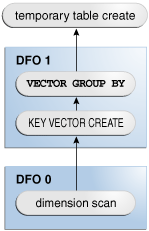
Description of "Figure 5-2 Phase 1 of In-Memory Aggregation"
-
-
Process the fact table.
-
Process all the joins and aggregations using the key vectors created in the preceding phase.
-
Join back the results to each temporary table.
Table 5-0 illustrates phase 2 in a join of the fact table with two dimensions. In DFO 0, the database performs a full scan of the fact table, and then uses the key vectors for each dimension to filter out nonmatching rows. DFO 2 joins the results of DFO 0 with DFO 1. DFO 4 joins the result of DFO 2 with DFO 3.
Figure 5-3 Phase 2 of In-Memory Aggregation
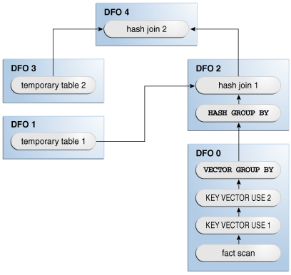
Description of "Figure 5-3 Phase 2 of In-Memory Aggregation"
-
5.7.3 Controls for In-Memory Aggregation
VECTOR GROUP BY aggregation does not involve any new SQL or public initialization parameters. You can use the following pairs of hints:
-
Query block hints
VECTOR_TRANSFORMenables the vector transformation on the specified query block, regardless of costing.NO_VECTOR_TRANSFORMdisables the vector transformation from engaging on the specified query block. -
Table hints
You can use the following pairs of hints:
-
VECTOR_TRANSFORM_FACTincludes the specifiedFROMexpressions in the fact table generated by the vector transformation.NO_VECTOR_TRANSFORM_FACTexcludes the specifiedFROMexpressions from the fact table generated by the vector transformation. -
VECTOR_TRANSFORM_DIMSincludes the specifiedFROMexpressions in enabled dimensions generated by the vector transformation.NO_VECTOR_TRANSFORM_DIMSexcludes the specified from expressions from enabled dimensions generated by the vector transformation.
-
See Also:
Oracle Database SQL Language Reference to learn more about theVECTOR_TRANSFORM_FACT and VECTOR_TRANSFORM_DIMS hints5.7.4 In-Memory Aggregation: Scenario
This section gives a conceptual example of how VECTOR GROUP BY aggregation works. The scenario does not use the sample schema tables or show an actual execution plan.
This section contains the following topics:
-
Step 1: Key Vector and Temporary Table Creation for geography Dimension
-
Step 2: Key Vector and Temporary Table Creation for products Dimension
5.7.4.1 Sample Analytic Query of a Star Schema
This sample star schema in this scenario contains the sales_online fact table and two dimension tables: geography and products. Each row in geography is uniquely identified by the geog_id column. Each row in products is uniquely identified by the prod_id column. Each row in sales_online is uniquely identified by the geog_id, prod_id, and amount sold.
Table 5-1 Sample Rows in geography Table
| country | state | city | geog_id |
|---|---|---|---|
|
USA |
WA |
seattle |
2 |
|
USA |
WA |
spokane |
3 |
|
USA |
CA |
SF |
7 |
|
USA |
CA |
LA |
8 |
Table 5-2 Sample Rows in products Table
| manuf | category | subcategory | prod_id |
|---|---|---|---|
|
Acme |
sport |
bike |
4 |
|
Acme |
sport |
ball |
3 |
|
Acme |
electric |
bulb |
1 |
|
Acme |
electric |
switch |
8 |
Table 5-3 Sample Rows in sales_online Table
| prod_id | geog_id | amount |
|---|---|---|
|
8 |
1 |
100 |
|
9 |
1 |
150 |
|
8 |
2 |
100 |
|
4 |
3 |
110 |
|
2 |
30 |
130 |
|
6 |
20 |
400 |
|
3 |
1 |
100 |
|
1 |
7 |
120 |
|
3 |
8 |
130 |
|
4 |
3 |
200 |
A manager asks the business question, "How many Acme products in each subcategory were sold online in Washington, and how many were sold in California?" To answer this question, an analytic query of the sales_online fact table joins the products and geography dimension tables as follows:
SELECT p.category, p.subcategory, g.country, g.state, SUM(s.amount)
FROM   sales_online s, products p, geography g
WHERE  s.geog_id = g.geog_id
AND    s.prod_id = p.prod_id
AND    g.state IN ('WA','CA')
AND    p.manuf = 'ACME'
GROUP BY category, subcategory, country, state
5.7.4.2 Step 1: Key Vector and Temporary Table Creation for geography Dimension
In the first phase of VECTOR GROUP BY aggregation for this query, the database creates a dense grouping key for each city/state combination for cities in the states of Washington or California. In Table 5-6, the 1 is the USA,WA grouping key, and the 2 is the USA,CA grouping key.
Table 5-4 Dense Grouping Key for geography
| country | state | city | geog_id | dense_gr_key_geog |
|---|---|---|---|---|
|
USA |
WA |
seattle |
2 |
1 |
|
USA |
WA |
spokane |
3 |
1 |
|
USA |
CA |
SF |
7 |
2 |
|
USA |
CA |
LA |
8 |
2 |
A key vector for the geography table looks like the array represented by the final column in Table 5-5. The values are the geography dense grouping keys. Thus, the key vector indicates which rows in sales_online meet the geography.state filter criteria (a sale made in the state of CA or WA) and which country/state group each row belongs to (either the USA,WA group or USA,CA group).
| prod_id | geog_id | amount | key vector for geography |
|---|---|---|---|
|
8 |
1 |
100 |
0 |
|
9 |
1 |
150 |
0 |
|
8 |
2 |
100 |
1 |
|
4 |
3 |
110 |
1 |
|
2 |
30 |
130 |
0 |
|
6 |
20 |
400 |
0 |
|
3 |
1 |
100 |
0 |
|
1 |
7 |
120 |
2 |
|
3 |
8 |
130 |
2 |
|
4 |
3 |
200 |
1 |
Internally, the database creates a temporary table similar to the following:
CREATE TEMPORARY TABLE tt_geography AS
SELECT MAX(country), MAX(state), KEY_VECTOR_CREATE(...) dense_gr_key_geog
FROM   geography
WHERE  state IN ('WA','CA')
GROUP BY country, state
Table 5-6 shows rows in the tt_geography temporary table. The dense grouping key for the USA,WA combination is 1, and the dense grouping key for the USA,CA combination is 2.
5.7.4.3 Step 2: Key Vector and Temporary Table Creation for products Dimension
The database creates a dense grouping key for each distinct category/subcategory combination of an Acme product. For example, in Table 5-7, the 4 is dense grouping key for an Acme electric switch.
Table 5-7 Sample Rows in products Table
| manuf | category | subcategory | prod_id | dense_gr_key_prod |
|---|---|---|---|---|
|
Acme |
sport |
bike |
4 |
1 |
|
Acme |
sport |
ball |
3 |
2 |
|
Acme |
electric |
bulb |
1 |
3 |
|
Acme |
electric |
switch |
8 |
4 |
A key vector for the products table might look like the array represented by the final column in Table 5-8. The values represent the products dense grouping key. For example, the 4 represents the online sale of an Acme electric switch. Thus, the key vector indicates which rows in sales_online meet the products filter criteria (a sale of an Acme product).
| prod_id | geog_id | amount | key vector for products |
|---|---|---|---|
|
8 |
1 |
100 |
4 |
|
9 |
1 |
150 |
0 |
|
8 |
2 |
100 |
4 |
|
4 |
3 |
110 |
1 |
|
2 |
30 |
130 |
0 |
|
6 |
20 |
400 |
0 |
|
3 |
1 |
100 |
2 |
|
1 |
7 |
120 |
3 |
|
3 |
8 |
130 |
2 |
|
4 |
3 |
200 |
1 |
Internally, the database creates a temporary table similar to the following:
CREATE TEMPORTARY TABLE tt_products AS
SELECT MAX(category), MAX(subcategory), KEY_VECTOR_CREATE(...) dense_gr_key_prod
FROM   products
WHERE  manuf = 'ACME'
GROUP BY category, subcategory
Table 5-9 shows rows in this temporary table.
5.7.4.4 Step 3: Key Vector Query Transformation
The database now enters the phase of processing the fact table. The optimizer transforms the original query into the following equivalent query, which accesses the key vectors:
SELECT KEY_VECTOR_PROD(prod_id),
       KEY_VECTOR_GEOG(geog_id),
       SUM(amount)
FROM   sales_online
WHERE  KEY_VECTOR_PROD_FILTER(prod_id) IS NOT NULL
AND    KEY_VECTOR_GEOG_FILTER(geog_id) IS NOT NULL
GROUP BY KEY_VECTOR_PROD(prod_id), KEY_VECTOR_GEOG(geog_id)
The preceding transformation is not an exact rendition of the internal SQL, which is much more complicated, but a conceptual representation designed to illustrate the basic concept.
5.7.4.5 Step 4: Row Filtering from Fact Table
The goal in this phase is to obtain the amount sold for each combination of grouping keys. The database uses the key vectors to filter out unwanted rows from the fact table. In Table 5-10, the first three columns represent the sales_online table. The last two columns provide the dense grouping keys for the geography and products tables.
Table 5-10 Dense Grouping Keys for the sales_online Table
| prod_id | geog_id | amount | dense_gr_key_prod | dense_gr_key_geog |
|---|---|---|---|---|
|
7 |
1 |
100 |
4 |
|
|
9 |
1 |
150 |
||
|
8 |
2 |
100 |
4 |
1 |
|
4 |
3 |
110 |
1 |
1 |
|
2 |
30 |
130 |
||
|
6 |
20 |
400 |
||
|
3 |
1 |
100 |
2 |
|
|
1 |
7 |
120 |
3 |
2 |
|
3 |
8 |
130 |
2 |
2 |
|
4 |
3 |
200 |
1 |
1 |
As shown in Table 5-11, the database retrieves only those rows from sales_online with non-null values for both dense grouping keys, indicating rows that satisfy all the filtering criteria.
5.7.4.6 Step 5: Aggregation Using an Array
The database uses a multidimensional array to perform the aggregation. In Table 5-12, the geography grouping keys are horizontal, and the products grouping keys are vertical. The database adds the values in the intersection of each dense grouping key combination. For example, for the intersection of the geography grouping key 1 and the products grouping key 1, the sum of 110 and 200 is 310.
5.7.4.7 Step 6: Join Back to Temporary Tables
In the final stage of processing, the database uses the dense grouping keys to join back the rows to the temporary tables to obtain the names of the regions and categories. The results look as follows:
CATEGORY SUBCATEGORY COUNTRY STATE AMOUNT
-------- ----------- ------- ----- ------
electric bulb        USA     CA    120
electric switch      USA     WA    100
sport    ball        USA     CA    130
sport    bike        USA     WA    310
5.7.5 In-Memory Aggregation: Example
The following query of the sh tables answers the business question "How many products were sold in each category in each calendar year?"
SELECT t.calendar_year, p.prod_category, SUM(quantity_sold)
FROM   times t, products p, sales s
WHERE  t.time_id = s.time_id
AND    p.prod_id = s.prod_id
GROUP BY t.calendar_year, p.prod_category;
Example 5-13 shows the execution plan contained in the current cursor. Steps 4 and 8 show the creation of the key vectors for the dimension tables times and products. Steps 17 and 18 show the use of the previously created key vectors. Steps 3, 7, and 15 show the VECTOR GROUP BY operations.
Example 5-13 VECTOR GROUP BY Execution Plan
SQL_ID  0yxqj2nq8p9kt, child number 0
-------------------------------------
SELECT t.calendar_year, p.prod_category, SUM(quantity_sold) FROM
times t, products p, sales f WHERE  t.time_id = f.time_id AND
p.prod_id   = f.prod_id GROUP BY t.calendar_year, p.prod_category

Plan hash value: 2377225738

----------------------------------------------------------------------------------------------------------------
|Id | Operation                            | Name                      |Rows|Bytes|Cost(%CPU)|Time|Pstart|Pstop|
----------------------------------------------------------------------------------------------------------------
|  0| SELECT STATEMENT                     |                           |    |     |285 (100)|        |   |    |
|  1|  TEMP TABLE TRANSFORMATION           |                           |    |     |         |        |   |    |
|  2|   LOAD AS SELECT                     | SYS_TEMP_0FD9D6644_11CBE8 |    |     |         |        |   |    |
|  3|    VECTOR GROUP BY                   |                           |   5|  80 |  3 (100)|00:00:01|   |    |
|  4|     KEY VECTOR CREATE BUFFERED       | :KV0000                   |1826|29216|  3 (100)|00:00:01|   |    |
|  5|      TABLE ACCESS INMEMORY FULL      | TIMES                     |1826|21912|  1 (100)|00:00:01|   |    |
|  6|   LOAD AS SELECT                     | SYS_TEMP_0FD9D6645_11CBE8 |    |     |         |        |   |    |
|  7|    VECTOR GROUP BY                   |                           |   5| 125 |  1 (100)|00:00:01|   |    |
|  8|     KEY VECTOR CREATE BUFFERED       | :KV0001                   |  72| 1800|  1 (100)|00:00:01|   |    |
|  9|      TABLE ACCESS INMEMORY FULL      | PRODUCTS                  |  72| 1512|  0   (0)|        |   |    |
| 10|   HASH GROUP BY                      |                           |  18| 1440|282  (99)|00:00:01|   |    |
|*11|    HASH JOIN                         |                           |  18| 1440|281  (99)|00:00:01|   |    |
|*12|     HASH JOIN                        |                           |  18| 990 |278 (100)|00:00:01|   |    |
| 13|      TABLE ACCESS FULL               | SYS_TEMP_0FD9D6644_11CBE8 |   5|  80 |  2   (0)|00:00:01|   |    |
| 14|      VIEW                            | VW_VT_AF278325            |  18| 702 |276 (100)|00:00:01|   |    |
| 15|       VECTOR GROUP BY                |                           |  18| 414 |276 (100)|00:00:01|   |    |
| 16|        HASH GROUP BY                 |                           |  18| 414 |276 (100)|00:00:01|   |    |
| 17|         KEY VECTOR USE               | :KV0000                   |918K|  20M|276 (100)|00:00:01|   |    |
| 18|          KEY VECTOR USE              | :KV0001                   |918K|  16M|272 (100)|00:00:01|   |    |
| 19|           PARTITION RANGE ALL        |                           |918K|  13M|257 (100)|00:00:01|  1|  28|
| 20|            TABLE ACCESS INMEMORY FULL| SALES                     |918K|  13M|257 (100)|00:00:01|  1|  28|
| 21|     TABLE ACCESS FULL                | SYS_TEMP_0FD9D6645_11CBE8 |  5 |  125|  2   (0)|00:00:01|   |    |
----------------------------------------------------------------------------------------------------------------

Predicate Information (identified by operation id):
---------------------------------------------------

  11 - access("ITEM_10"=INTERNAL_FUNCTION("C0") AND "ITEM_11"="C2")
  12 - access("ITEM_8"=INTERNAL_FUNCTION("C0") AND "ITEM_9"="C2")

Note
-----
   - vector transformation used for this statement

45 rows selected.
5.8 Table Expansion
In table expansion, the optimizer generates a plan that uses indexes on the read-mostly portion of a partitioned table, but not on the active portion of the table. This section contains the following topics:
5.8.1 Purpose of Table Expansion
Table expansion is useful because of the following facts:
-
Index-based plans can improve performance dramatically.
-
Index maintenance causes overhead to DML.
-
In many databases, only a small portion of the data is actively updated through DML.
Table expansion takes advantage of index-based plans for tables that have high update volume. You can configure a table so that an index is only created on the read-mostly portion of the data, and does not suffer the overhead burden of index maintenance on the active portions of the data. Thus, table expansion reaps the benefit of improved performance without suffering the ill effects of index maintenance.
5.8.2 How Table Expansion Works
Table partitioning makes table expansion possible. If a local index exists on a partitioned table, then the optimizer can mark the index as unusable for specific partitions. In effect, some partitions are not indexed.
In table expansion, the optimizer transforms the query into a UNION ALL statement, with some subqueries accessing indexed partitions and other subqueries accessing unindexed partitions. The optimizer can choose the most efficient access method available for a partition, regardless of whether it exists for all of the partitions accessed in the query.
The optimizer does not always choose table expansion:
-
Table expansion is cost-based.
While the database accesses each partition of the expanded table only once across all branches of the
UNION ALL, any tables that the database joins to it are accessed in each branch. -
Semantic issues may render expansion invalid.
For example, a table appearing on the right side of an outer join is not valid for table expansion.
You can control table expansion with the hint EXPAND_TABLE hint. The hint overrides the cost-based decision, but not the semantic checks.
See Also:
"Influencing the Optimizer with Hints"5.8.3 Table Expansion: Scenario
The optimizer keeps track of which partitions must be accessed from each table, based on predicates that appear in the query. Partition pruning enables the optimizer to use table expansion to generate more optimal plans.
This scenario assumes the following:
-
You want to run a star query against the
sh.salestable, which is range-partitioned on thetime_idcolumn. -
You want to disable indexes on specific partitions to see the benefits of table expansion.
To use table expansion:
-
Run the following query:
SELECT * FROM sales WHERE time_id >= TO_DATE('2000-01-01 00:00:00', 'SYYYY-MM-DD HH24:MI:SS') AND prod_id = 38; -
Explain the plan by querying
DBMS_EXPLAN:SET LINESIZE 150 SET PAGESIZE 0 SELECT * FROM TABLE(DBMS_XPLAN.DISPLAY_CURSOR(format => 'BASIC,PARTITION'));
As shown in the
PstartandPstopcolumns in the following plan, the optimizer determines from the filter that only 16 of the 28 partitions in the table must be accessed:Plan hash value: 3087065703 ------------------------------------------------------------------------------- | Id| Operation | Name |Pstart|Pstop| ------------------------------------------------------------------------------- | 0 | SELECT STATEMENT | | | | | 1 | PARTITION RANGE ITERATOR | | 13 | 28 | | 2 | TABLE ACCESS BY LOCAL INDEX ROWID BATCHED| SALES | 13 | 28 | | 3 | BITMAP CONVERSION TO ROWIDS | | | | |*4 | BITMAP INDEX SINGLE VALUE | SALES_PROD_BIX| 13 | 28 | ------------------------------------------------------------------------------- Predicate Information (identified by operation id): --------------------------------------------------- 4 - access("PROD_ID"=38)After the optimizer has determined the partitions to be accessed, it considers any index that is usable on all of those partitions. In the preceding plan, the optimizer chose to use the
sales_prod_bixbitmap index. -
Disable the index on the
SALES_1995partition of thesalestable:ALTER INDEX sales_prod_bix MODIFY PARTITION sales_1995 UNUSABLE;
The preceding DDL disables the index on partition 1, which contains all sales from before 1996.
Note:
You can obtain the partition information by querying theUSER_IND_PARTITIONSview. -
Execute the query of sales again, and then query
DBMS_XPLANto obtain the plan.The output shows that the plan did not change:
Plan hash value: 3087065703

-------------------------------------------------------------------------------
| Id| Operation                                  | Name           |Pstart|Pstop
-------------------------------------------------------------------------------
| 0 | SELECT STATEMENT                           |                |      |    |
| 1 |  PARTITION RANGE ITERATOR                  |                |  13  | 28 |
| 2 |   TABLE ACCESS BY LOCAL INDEX ROWID BATCHED| SALES          |  13  | 28 |
| 3 |    BITMAP CONVERSION TO ROWIDS             |                |      |    |
|*4 |     BITMAP INDEX SINGLE VALUE              | SALES_PROD_BIX |  13  | 28 |
-------------------------------------------------------------------------------

Predicate Information (identified by operation id):
---------------------------------------------------

   4 - access("PROD_ID"=38)
The plan is the same because the disabled index partition is not relevant to the query. If all partitions that the query accesses are indexed, then the database can answer the query using the index. Because the query only accesses partitions 16 through 28, disabling the index on partition 1 does not affect the plan.
-
Disable the indexes for partition 28 (
SALES_Q4_2003), which is a partition that the query needs to access:ALTER INDEX sales_prod_bix MODIFY PARTITION sales_q4_2003 UNUSABLE; ALTER INDEX sales_time_bix MODIFY PARTITION sales_q4_2003 UNUSABLE;
By disabling the indexes on a partition that the query does need to access, the query can no longer use this index (without table expansion).
-
Query the plan using
DBMS_EXPLAN.As shown in the following plan, the optimizer does not use the index:
Plan hash value: 3087065703

-------------------------------------------------------------------------------
| Id| Operation                                  | Name           |Pstart|Pstop
-------------------------------------------------------------------------------
| 0 | SELECT STATEMENT                           |                |      |    |
| 1 |  PARTITION RANGE ITERATOR                  |                |  13  | 28 |
|*2 |   TABLE ACCESS FULL                        | SALES          |  13  | 28 |
-------------------------------------------------------------------------------

Predicate Information (identified by operation id):
---------------------------------------------------
   2 - access("PROD_ID"=38)
In the preceding example, the query accesses 16 partitions. On 15 of these partitions, an index is available, but no index is available for the final partition. Because the optimizer has to choose one access path or the other, the optimizer cannot use the index on any of the partitions.
-
With table expansion, the optimizer rewrites the original query as follows:
SELECT *
FROM   sales
WHERE  time_id >= TO_DATE('2000-01-01 00:00:00', 'SYYYY-MM-DD HH24:MI:SS')
AND    time_id <  TO_DATE('2003-10-01 00:00:00', 'SYYYY-MM-DD HH24:MI:SS')
AND    prod_id = 38
UNION ALL
SELECT *
FROM   sales
WHERE  time_id >= TO_DATE('2003-10-01 00:00:00', 'SYYYY-MM-DD HH24:MI:SS')
AND    time_id < TO_DATE('2004-01-01 00:00:00', 'SYYYY-MM-DD HH24:MI:SS')
AND    prod_id = 38;
In the preceding query, the first query block in the
UNION ALLaccesses the partitions that are indexed, while the second query block accesses the partition that is not. The two subqueries enable the optimizer to choose to use the index in the first query block, if it is more optimal than using a table scan of all of the partitions that are accessed. -
Query the plan using
DBMS_EXPLAN.The plan appears as follows:
Plan hash value: 2120767686

-------------------------------------------------------------------------------
| Id  | Operation                                   | Name       |Pstart|Pstop|
-------------------------------------------------------------------------------
|  0 | SELECT STATEMENT                             |                |    |   |
|  1 |  VIEW                                        | VW_TE_2        |    |   |
|  2 |   UNION-ALL                                  |                |    |   |
|  3 |    PARTITION RANGE ITERATOR                  |                | 13 | 27|
|  4 |     TABLE ACCESS BY LOCAL INDEX ROWID BATCHED| SALES          | 13 | 27|
|  5 |      BITMAP CONVERSION TO ROWIDS             |                |    |   |
|* 6 |       BITMAP INDEX SINGLE VALUE              | SALES_PROD_BIX | 13 | 27|
|  7 |    PARTITION RANGE SINGLE                    |                | 28 | 28|
|* 8 |     TABLE ACCESS FULL                        | SALES          | 28 | 28|
-------------------------------------------------------------------------------

Predicate Information (identified by operation id):
---------------------------------------------------

   6 - access("PROD_ID"=38)
   8 - filter("PROD_ID"=38)
As shown in the preceding plan, the optimizer uses a
UNION ALLfor two query blocks (Step 2). The optimizer chooses an index to access partitions 13 to 27 in the first query block (Step 6). Because no index is available for partition 28, the optimizer chooses a full table scan in the second query block (Step 8).
5.8.4 Table Expansion and Star Transformation: Scenario
Star transformation enables specific types of queries to avoid accessing large portions of big fact tables (see "Star Transformation"). Star transformation requires defining several indexes, which in an actively updated table can have overhead. With table expansion, you can define indexes on only the inactive partitions so that the optimizer can consider star transformation on only the indexed portions of the table.
This scenario assumes the following:
-
You query the same schema used in "Star Transformation: Scenario".
-
The last partition of
salesis actively being updated, as is often the case with time-partitioned tables. -
You want the optimizer to take advantage of table expansion.
To take advantage of table expansion in a star query:
-
Disable the indexes on the last partition as follows:
ALTER INDEX sales_channel_bix MODIFY PARTITION sales_q4_2003 UNUSABLE;
ALTER INDEX sales_cust_bix MODIFY PARTITION sales_q4_2003 UNUSABLE;
-
Execute the following star query:
SELECT t.calendar_quarter_desc, SUM(s.amount_sold) sales_amount FROM sales s, times t, customers c, channels ch WHERE s.time_id = t.time_id AND s.cust_id = c.cust_id AND s.channel_id = ch.channel_id AND c.cust_state_province = 'CA' AND ch.channel_desc = 'Internet' AND t.calendar_quarter_desc IN ('1999-01','1999-02') GROUP BY t.calendar_quarter_desc; -
Query the cursor using
DBMS_XPLAN, which shows the following plan:------------------------------------------------------------------------------- | Id | Operation | Name | Pstart| Pstop | ------------------------------------------------------------------------------- | 0 | SELECT STATEMENT | | | | | 1 | HASH GROUP BY | | | | | 2 | VIEW | VW_TE_14 | | | | 3 | UNION-ALL | | | | | 4 | HASH JOIN | | | | | 5 | TABLE ACCESS FULL | TIMES | | | | 6 | VIEW | VW_ST_1319B6D8 | | | | 7 | NESTED LOOPS | | | | | 8 | PARTITION RANGE SUBQUERY | |KEY(SQ)|KEY(SQ)| | 9 | BITMAP CONVERSION TO ROWIDS| | | | | 10 | BITMAP AND | | | | | 11 | BITMAP MERGE | | | | | 12 | BITMAP KEY ITERATION | | | | | 13 | BUFFER SORT | | | | | 14 | TABLE ACCESS FULL | CHANNELS | | | | 15 | BITMAP INDEX RANGE SCAN| SALES_CHANNEL_BIX |KEY(SQ)|KEY(SQ)| | 16 | BITMAP MERGE | | | | | 17 | BITMAP KEY ITERATION | | | | | 18 | BUFFER SORT | | | | | 19 | TABLE ACCESS FULL | TIMES | | | | 20 | BITMAP INDEX RANGE SCAN| SALES_TIME_BIX |KEY(SQ)|KEY(SQ)| | 21 | BITMAP MERGE | | | | | 22 | BITMAP KEY ITERATION | | | | | 23 | BUFFER SORT | | | | | 24 | TABLE ACCESS FULL | CUSTOMERS | | | | 25 | BITMAP INDEX RANGE SCAN| SALES_CUST_BIX |KEY(SQ)|KEY(SQ)| | 26 | TABLE ACCESS BY USER ROWID | SALES | ROWID | ROWID | | 27 | NESTED LOOPS | | | | | 28 | NESTED LOOPS | | | | | 29 | NESTED LOOPS | | | | | 30 | NESTED LOOPS | | | | | 31 | PARTITION RANGE SINGLE | | 28 | 28 | | 32 | TABLE ACCESS FULL | SALES | 28 | 28 | | 33 | TABLE ACCESS BY INDEX ROWID| CHANNELS | | | | 34 | INDEX UNIQUE SCAN | CHANNELS_PK | | | | 35 | TABLE ACCESS BY INDEX ROWID | CUSTOMERS | | | | 36 | INDEX UNIQUE SCAN | CUSTOMERS_PK | | | | 37 | INDEX UNIQUE SCAN | TIMES_PK | | | | 38 | TABLE ACCESS BY INDEX ROWID | TIMES | | | -------------------------------------------------------------------------------
The preceding plan uses table expansion. The
UNION ALLbranch that is accessing every partition except the last partition uses star transformation. Because the indexes on partition 28 are disabled, the database accesses the final partition using a full table scan.
5.9 Join Factorization
In the cost-based transformation known as join factorization, the optimizer can factorize common computations from branches of a UNION ALL query.
This section contains the following topics:
5.9.1 Purpose of Join Factorization
UNION ALL queries are common in database applications, especially in data integration applications. Often, branches in a UNION ALL query refer to the same base tables. Without join factorization, the optimizer evaluates each branch of a UNION ALL query independently, which leads to repetitive processing, including data access and joins. Join factorization transformation can share common computations across the UNION ALL branches. Avoiding an extra scan of a large base table can lead to a huge performance improvement.
5.9.2 How Join Factorization Works
Join factorization can factorize multiple tables and from more than two UNION ALL branches. Join factorization is best explained through examples. Example 5-14 shows a query of four tables and two UNION ALL branches.
SELECT t1.c1, t2.c2
FROM   t1, t2, t3
WHERE  t1.c1 = t2.c1
AND    t1.c1 > 1
AND    t2.c2 = 2
AND    t2.c2 = t3.c2
UNION ALL
SELECT t1.c1, t2.c2
FROM   t1, t2, t4
WHERE  t1.c1 = t2.c1
AND    t1.c1 > 1
AND    t2.c3 = t4.c3
In Example 5-14, table t1 appears in both UNION ALL branches, as does the filter predicate t1.c1 > 1 and the join predicate t1.c1 = t2.c1. Nevertheless, without any transformation, the database must perform the scan and the filtering on table t1 twice, one time for each branch. Example 5-15 uses join factorization to transform the query in Example 5-14.
SELECT t1.c1, VW_JF_1.item_2
FROM   t1, (SELECT t2.c1 item_1, t2.c2 item_2
            FROM   t2, t3
            WHERE  t2.c2 = t3.c2
            AND    t2.c2 = 2
            UNION ALL
            SELECT t2.c1 item_1, t2.c2 item_2
            FROM   t2, t4
            WHERE  t2.c3 = t4.c3) VW_JF_1
WHERE  t1.c1 = VW_JF_1.item_1
AND    t1.c1 > 1
In Example 5-15, table t1 is factorized. Thus, the database performs the table scan and the filtering on t1 only one time. If t1 is large, then this factorization avoids the huge performance cost of scanning and filtering t1 twice.
Note:
If the branches in aUNION ALL query have clauses that use the DISTINCT function, then join factorization is not valid.5.9.3 Factorization and Join Orders: Scenario
A benefit of join factorization is that it can create more possibilities for join orders. In Example 5-16, view V is same as the query in Example 5-14.
Example 5-16 Query Involving Five Tables
SELECT *
FROM   t5, (SELECT t1.c1, t2.c2
            FROM   t1, t2, t3
            WHERE  t1.c1 = t2.c1
            AND    t1.c1 > 1
            AND    t2.c2 = 2
            AND    t2.c2 = t3.c2
            UNION ALL
            SELECT t1.c1, t2.c2
            FROM   t1, t2, t4
            WHERE  t1.c1 = t2.c1
            AND    t1.c1 > 1
            AND    t2.c3 = t4.c3) V
WHERE  t5.c1 = V.c1
Before join factorization, the database must join t1, t2, and t3 before joining them with t5. But if join factorization factorizes t1 from view V, as shown in Example 5-17, then the database can join t1 with t5.
Example 5-17 Factorization of t1 from View V
SELECT *
FROM   t5, ( SELECT t1.c1, VW_JF_1.item_2
             FROM   t1, (SELECT t2.c1 item_1, t2.c2 item_2
                         FROM   t2, t3
                         WHERE  t2.c2 = t3.c2
                         AND    t2.c2 = 2
                         UNION ALL
                         SELECT t2.c1 item_1, t2.c2 item_2
                         FROM   t2, t4
                         WHERE  t2.c3 = t4.c3) VW_JF_1
             WHERE  t1.c1 = VW_JF_1.item_1
             AND    t1.c1 > 1 )
WHERE  t5.c1 = V.c1
Example 5-18 shows the same query as Example 5-17, but with the view definition removed so that the factorization is easier to see.
Example 5-18 Factorization of t1 from View V
SELECT *
FROM   t5, (SELECT t1.c1, VW_JF_1.item_2
            FROM   t1, VW_JF_1
            WHERE  t1.c1 = VW_JF_1.item_1
            AND    t1.c1 > 1)
WHERE  t5.c1 = V.c1
The query transformation in Example 5-17 opens up new join orders. However, join factorization imposes specific join orders. For example, in Example 5-17, tables t2 and t3 appear in the first branch of the UNION ALL query in view VW_JF_1. The database must join t2 with t3 before it can join with t1, which is not defined within the VW_JF_1 view. The imposed join order may not necessarily be the best join order. For this reason, the optimizer performs join factorization using the cost-based transformation framework. The optimizer calculate the cost of the plans with and without join factorization, and then chooses the cheapest plan.
5.9.4 Factorization of Outer Joins: Scenario
The database supports join factorization of outer joins, antijoins, and semijoins, but only for the right tables in such joins. For example, join factorization can transform the query in Example 5-19 by factorizing t2.
SELECT t1.c2, t2.c2
FROM   t1, t2
WHERE  t1.c1 = t2.c1(+)
AND    t1.c1 = 1
UNION ALL
SELECT t1.c2, t2.c2
FROM   t1, t2
WHERE  t1.c1 = t2.c1(+)
AND    t1.c1 = 2
Example 5-20 shows the factorized query.