a side-by-side reference sheet
arithmetic and logic | strings | regexes | dates and time | arrays | dictionaries | functions | execution control | files
libraries | reflection
mapping and filtering | aggregating | joining | sorting | contact
| sql | awk | pig | |
|---|---|---|---|
| version used |
PostgreSQL 9.0 | 20070501 | 0.9 |
| show version |
$ psql --version | $ awk --version | $ pig --version |
| interpreter |
$ psql -f foo.sql | $ awk -f foo.awk bar.txt | $ pig -f foo.pig |
| repl |
$ psql | none | $ pig -x local |
| input data format | multiple tables defined by create table statements | single field and record delimited file. By default fields are delimited by whitespace and records by newlines | multiple files. Default loading function is PigStorage and default delimiter is tab |
| statement separator | ; | ; or newline | ; and newline when using REPL |
| block delimiter | none in SQL; PL/SQL uses keywords to delimit blocks | { } | |
| to-end-of-line comment | -- comment | # comment | -- comment |
| comment out multiple lines | none | none | /* comment another comment */ |
| case sensitive? | no | yes | functions and aliases are case sensitive; commands and operators are not |
| quoted identifier | create table "select" ( "foo bar" int); MySQL: create table `select` ( `foo bar` int ); |
none | none |
| null |
null | "" | null |
| null test |
foo is null | foo == "" | in filter clause: is null |
| coalesce |
coalesce(foo, 0) | foo is null ? 0 : foo | |
| arithmetic and logic | |||
| sql | awk | pig | |
| true and false |
true false | 1 0 | none |
| falsehoods | false the predicate of a where clause evaluates as false if it contains a null |
0 "" | none; the first operand of a conditional expression must be a comparison operator expression |
| logical operators | and or not | && || ! | in filter clause: and or not |
| integer types | smallint 2 bytes int 4 bytes bigint 8 bytes |
variables are untyped | int 4 bytes long 8 bytes |
| float and fixed types | float 4 bytes double 8 bytes numeric(precision, scale) |
variables are untyped | float 4 bytes double 8 bytes |
| conditional expression | case when x > 0 then x else -x end | x > 0 ? x : -x | x > 0 ? x : -x |
| comparison operators | = != > < >= <= | == != > < >= <= | == != > < >= <= |
| arithmetic operators | + - * / % ^ | + - * / % ^ | + - * / % |
| integer division | 13 / 5 | int(13 / 5) | 13 / 5 |
| float division |
cast(13 as float) / 5 | 13 / 5 | 1.0 * 13 / 5 |
| arithmetic functions | sqrt exp ln sin cos tan asin acos atan atan2 | sqrt exp log sin cos none none none none atan2 | SQRT EXP LOG SIN COS TAN ASIN ACOS ATAN none |
| arithmetic truncation | cast(2.7 as int) round(2.7) ceil(2.7) floor(2.7) abs(-2.7) |
int(2.7) | (int)2.7 ROUND(2.7) CEIL(2.7) FLOOR(2.7) ABS(-2.7) |
| random float |
random() | rand() | RANDOM() |
| strings | |||
| sql | awk | pig | |
| types | text varchar(n) char(n) |
variables are untyped | chararray bytearray |
| literal |
'don''t say "no"' PostgreSQL escape literal: E'don\'t say "no"' |
"don't say \"no\"" | 'don\'t say "no"' |
| length |
length('lorem ipsum') | length("lorem ipsum") | SIZE('lorem ipsum') |
| escapes | no backslash escapes in SQL standard string literals in PostgreSQL escape literals: \b \f \n \r \t \ooo \xhh \uhhhh \uhhhhhhhh |
\\ \" \a \b \f \n \r \t \v \ooo \xhh | \n \t \uhhhh |
| concatenation |
'Hello' || ', ' || 'World!' | "Hello" ", " "World!" | CONCAT(CONCAT('Hello', ', '), 'World!') |
| split |
regexp_split_to_array('do re mi', ' ') | split("do re mi", a, " ") | STRSPLIT('do re mi', ' ') |
| case manipulation | upper('lorem') lower('LOREM') initcap('lorem') |
toupper("lorem") tolower("LOREM") none |
UPPER('lorem') LOWER('LOREM') UCFIRST('lorem') |
| strip | trim(' lorem ') ltrim(' lorem') rtrim('lorem ') |
TRIM(' lorem ') | |
| index of substring | index starts from 1; returns 0 if not found: strpos('lorem ipsum', 'ipsum') |
index starts from 1; returns 0 if not found: index("lorem ipsum", "ipsum") |
index starts from 0; returns -1 if not found: INDEXOF('lorem ipsum', 'ipsum', 0) |
| extract substring | substr('lorem ipsum', 7, 5) | substr("lorem ipsum", 7, 5) | SUBSTRING('lorem ipsum', 6, 11) |
| sprintf | select format('%s %s %s', 'foo', 7, 13.2); | sprintf("%s %d %f", "foo", 7, 13.2) | REGISTER /PATH/TO/piggybank-0.3-amzn.jar; DEFINE FORMAT org.apache.pig.piggybank.evaluation.string.FORMAT(); foo = FOREACH foo GENERATE FORMAT('%s %d %f', 'foo', 7, 13.2); |
| regular expressions | |||
| sql | awk | pig | |
| match | select * from pwt where name similar to 'r[a-z]+'; |
matching inside pattern: $1 ~ /^r[a-z]+/ { print $0 } matching inside action: { if (match($1, /^r[a-z]+$/)) print $0 } |
root_pwf = filter pwf by SIZE(REGEX_EXTRACT(name, '^(root)$',1)) > 0; |
| substitute |
select regexp_replace('foo bar', 'bar$', 'baz'); | s = "foo bar" sub(/bar$/, "baz", s) |
|
| extract subgroup | none | properties = FOREACH urls GENERATE FLATTEN(EXTRACT($0, '^https?://([^/]+)')) as host:chararray; | |
| dates and time | |||
| sql | awk | pig | |
| current date and time | now() | gawk: systime() |
REGISTER /PATH/TO/piggybank-0.3-amzn.jar; DEFINE DATE_TIME org.apache.pig.piggybank.evaluation.datetime.DATE_TIME(); bar = FOREACH foo GENERATE DATE_TIME('-00:00'); |
| datetime to string | to_char(now(), 'YYYY-MM-DD HH24:MI:SS') | gawk: strftime("%Y-%m-%d %H:%M:%S", systime()) |
REGISTER /PATH/TO/piggybank-0.3-amzn.jar; DEFINE FORMAT_DT org.apache.pig.piggybank.evaluation.datetime.FORMAT_DT(); baz = FOREACH bar GENERATE FORMAT_DT('yyyy-MM-dd HH::mm:ss', $0); |
| string to datetime | to_timestamp('2011-09-26 00:00:47', 'YYYY-MM-DD HH24:MI:SS') | gawk: mktime("2011 09 26 00 00 47") |
|
| arrays | |||
| sql | awk | pig | |
| literal | PostgreSQL: create temp table foo ( a int[] ); insert into foo values ( '{1,2,3}' ); |
none | one_row = LOAD '/tmp/one_line.txt'; foo = FOREACH one_row GENERATE (1,2,3); |
| size | PostgreSQL: select array_upper(a, 1) from foo; |
length(a) | bar = FOREACH foo GENERATE SIZE(a); |
| lookup | PostgreSQL: select a[1] from foo; |
a[0] | bar = FOREACH foo GENERATE a.$0; |
| update | |||
| iteration | for (i in a) print i, a[i] | ||
| dictionaries | |||
| sql | awk | pig | |
| literal | ['t'#1, 'f'#0] | ||
| functions | |||
| pl/sql | awk | pig | |
| define function | create or replace function add ( x int, y int ) returns int as $$ begin return x + y; end; $$ language plpgsql; |
can be defined at position of pattern-action statement: function add(x, y) { return x+y } |
in org/hpglot/Add.java: package org.hpglot; import java.io.IOException; import org.apache.pig.EvalFunc; import org.apache.pig.data.Tuple; public class Add extends EvalFunc<Integer> { @Override public Integer exec(Tuple input) throws IOException { Integer x, y; if (input == null || input.size() != 2) { throw new IOException("Takes 2 args"); } x = (Integer)input.get(0); y = (Integer)input.get(1); return x + y; } } how to compile: $ export CLASSPATH=$PIG_DIR/pig-0.9.0-core.jar $ javac org/hpglot/Add.java $ jar cf Add.jar org/hpglot |
| invoke function | select add(x, y) from foo; | { print add($1, $2) } | REGISTER Add.jar DEFINE ADD org.hpglot.Add(); foo = LOAD 'foo.txt' AS (x:int, y:int); bar = FOREACH foo GENERATE ADD(x, y); |
| drop function |
drop function add(integer, integer); | none | none |
| execution control | |||
| pl/sql | awk | pig | |
| if | if (!0) print "foo"; else print "bar" | none | |
| while | i = 0; while (i<5) print i++ | none | |
| for | for (i=0; i<5; i++) print i | none | |
| files | |||
| sql | awk | pig | |
| set field delimiter | $ grep -v '^#' /etc/passwd > /tmp/pw create table pwt ( name text, pw text, uid int, gid int, gecos text, home text, sh text ); copy pwt from '/tmp/pw' with delimiter ':'; |
BEGIN { FS=":" } | pwf = LOAD '/etc/passwd' USING PigStorage(':') AS (name:chararray, pw:chararray, uid:int, gid:int, gecos:chararray, home:chararray, sh:chararray); |
| write table to file | STORE foo INTO '/tmp/foo.tab'; | ||
| libraries | |||
| sql | awk | pig | |
| reflection | |||
| sql | awk | pig | |
| table schema | DESCRIBE foo; | ||
| mapping and filtering | |||
| sql | awk | pig | |
| select columns by name | select name, pw from pwt; | none | name_pw = foreach pwf generate name, pw; |
| select columns by position | none | { print $1, $2 } | name_pw = foreach pwf generate $0, $1; |
| select all columns | select * from pwt; | # prints input line: { print $0 } |
pwf2 = foreach pwf generate *; |
| rename columns | select uid as userid, gid as groupid from pwf; |
none | usergroups = foreach pwf generate uid as userid, gid as groupid; |
| filter rows | select * from pwt where name = 'root'; | $1 == "root" { print $0 } | pwf3 = filter pwf by name == 'root'; |
| split rows | split pwf into rootpwf if name == 'root', otherpwf if name != 'root'; | ||
| aggregating | |||
| sql | awk | pig | |
| select distinct | select distinct gid from pwt; | $ cat > gid.awk BEGIN { FS=":" } !/^#/ { print $4 } $ awk -f gid.awk /etc/passwd > /tmp/x $ sort -u /tmp/x |
gids1 = foreach pwf generate gid; gids2 = distinct gids1; |
| group by | select gid, count(*) from pwf group by gid; |
BEGIN { FS=":" } !/^#/ { $a[$4]++ } END { for (i in a) print i, a[i] } |
by_group = group pwf by gid; cnts = foreach by_group generate $0, COUNT($1); |
| group by multiple columns | select gid, sh, count(*) from pwf group by gid, sh; |
by_group = group pwf by (gid, sh); cnts = foreach by_group generate FLATTEN($0), COUNT($1); |
|
| aggregation functions | count sum min max avg stddev | COUNT SUM MIN MAX AVG none | |
| rank | |||
| quantile | |||
| joining | |||
| sql | join | pig | |
| inner join | create temp table gt ( name text, pw text, gid int, members text ); copy gt from '/etc/group' with delimiter ':'; select * from pwt join gt on pwt.gid = gt.gid; |
$ awk '!/^#/' /etc/passwd > /tmp/x $ sort -k4,4 -t: < /tmp/x > /tmp/pw $ awk '!/^#/' /etc/group > /tmp/y $ sort -k3,3 -t: < /tmp/y > /tmp/g $ join -t: -14 -23 /tmp/pw /tmp/g |
gf = load '/etc/group' using PigStorage(':') as (name:chararray, pw:chararray, gid:int, members:chararray); pwgf = join pwf by gid, gf by gid; |
| null treatment in joins | input relations with nulls for join values are omitted | no null value; empty strings are joinable values | input relations with nulls for join values are omitted |
| self join | select pwt1.name, pwt2.name from pwt as pwt1, pwt as pwt2 where pwt1.gid = pwt2.gid; |
$ join -t: -14 -24 /tmp/pw /tmp/pw | pwf2 = foreach pwf generate *; joined_by_gid = join pwf by gid, pwf2 by gid; name_pairs = foreach by_group generate pwf::name, pwf2::name; |
| left join | select * from customers c left join orders o on c.id = o.customer_id; |
$ join -t: -a1 -11 -22 /tmp/c /tmp/o | j = join customers by id left, orders by customer_id; |
| full join | select * from customers c full join orders o on c.id = o.customer_id; |
$ join -t: -a1 -a2 -11 -22 /tmp/c /tmp/o | j = join customers by id full, orders by customer_id; |
| cartesian join | create table files ( file text ); insert into files values ('a'), ('b'), ('c'), ('d'), ('e'), ('f'), ('g'), ('h'); create table ranks ( rank int ); insert into ranks values (1), (2), (3), (4), (5), (6), (7), (8); create table chessboard ( file text, rank int ); insert into chessboard select * from files, ranks; |
specify nonexistent join fields: $ join -12 -22 /tmp/f /tmp/r |
files = load '/tmp/files.txt' as (file:chararray); ranks = load '/tmp/ranks.txt' as (rank:int); chessboard = cross files, ranks; |
| sorting | |||
| sql | awk | pig | |
| order by | select name from pwt order by name; |
$ sort -k1 -t: /etc/passwd | names = foreach pwf generate name; ordered_names = order names by name; |
| order by multiple columns | |||
| limit | select name from pwt order by name limit 10; | first_ten = limit ordered_names 10; | |
| offset | select name from pwt order by name limit 10 offset 10; | ||
| ___________________________________________________________ | ___________________________________________________________ | ___________________________________________________________ | |
General Footnotes
versions used
The versions used for testing code in the reference sheet.
show version
How to get the version.
interpreter
How to run the interpreter on a script.
repl
How to invoke the REPL.
statement separator
The statement separator.
block delimiter
The delimiters used for blocks.
to-end-of-line comment
How to create a comment that ends at the next newline.
comment out mutliple lines
How to comment out multiple lines.
case sensitive?
Are identifiers which differ only by case treated as distinct identifiers?
quoted identifier
How to quote an identifier.
Quoting an identifier is a way to include characters which aren't normally permitted in an identifer.
In SQL quoting is also a way to refer to an identifier that would otherwise be interpreted as a reserved word
null
The null literal.
pig:
PigStorage, the default function for loading and persisting relations, represents a null value with an empty string. Null is distinct from an empty string since null == '' evaluates as false. Thus PigStorage cannot load or store an empty string.
null test
How to test whether an expression is null.
sql:
The expression null = null evaluates as null, which is a ternary boolean value distinct from true and false. Expressions built up from arithmetic operators or comparison operators which contain a null evaluate as null. When logical operators are involved, null behaves like the unknown value of Kleene logic.
coalesce
How to use the value of an expression, replacing it with an alternate value if it is null.
Arithmetic and Logic Footnotes
true and false
Literals for true and false.
falsehoods
Values which evaluate as false in a boolean context.
logical operators
The logical operators. Logical operators impose a boolean context on their arguments and return a boolean value.
integer types
sql:
Datatypes are database specific, but the mentioned types are provided by both PostgreSQL and MySQL.
awk:
Variables are untyped and implicit conversions are performed between numeric and string types.
The numeric literal for zero, 0, evaluates as false, but the string "0" evaluates as true. Hence we can infer that awk has at least two distinct data types.
float and fixed types
sql:
Datatypes are database specific, but the mentioned types are provided by both PostgreSQL and MySQL.
conditional expression
The syntax for a conditional expression.
comparison operations
The comparison operators, also known as the relational operators.
arithmetic operatorions
The arithmetic operators: addition, subtraction, multiplication, division, modulus, and exponentiation.
integer division
How to compute the quotient of two numbers. The quotient is always an integer.
float division
How to perform floating point division, even if the operands are integers.
arithmetic functions
The standard transcendental functions of mathematics.
arithmetic truncation
How to truncate floats to integers. The functions (1) round towards zero, (2) round to the nearest integer, (3) round towards positive infinity, and (4) round towards negative infinity. How to get the absolute value of a number is also illustrated.
random float
How to create a unit random float.
String Footnotes
types
The available string types.
pig:
A chararray is a string of Unicode characters. Like in Java the characters are UTF-16 encoded.
A bytearray is a string of bytes. Data imported into Pig is of type bytearray unless declared otherwise.
literal
The syntax for string literals.
sql:
MySQL also has double quoted string literals. PostgreSQL and most other database use double quotes for identifiers.
In a MySQL double quoted string double quote characters must be escaped with reduplication but single quote characters do not need to be escaped.
pig:
Single quoted string literals are of type chararray. There is no syntax for a bytearray literal.
length
How to get the length of a string.
escapes
Escape sequences which are available in string literals.
sql:
Here is a portable way to include a newline character in a SQL string:
select 'foo' || chr(10) || 'bar';
MySQL double and single quoted strings support C-style backslash escapes. Backslash escapes are not part of the SQL standard. Their interpretation can be disabled at the session level with
SET sql_mode='NO_BACKSLASH_ESCAPES';
concatenation
How to concatenate strings.
split
How to split a string into an array of substrings.
sql:
How to split a string into multiple rows of data:
=> create temp table foo ( bar text );
CREATE TABLE

=> insert into foo select regexp_split_to_table('do re mi', ' ');
INSERT 0 3
case manipulation
How to uppercase a string; how to lower case a string; how to capitalize the first character.
strip
How to remove whitesapce from the edges of a string.
index of substring
How to get the leftmost index of a substring in a string.
extract substring
How to extract a substring from a string.
sprintf
How to create a string from a format.
Regular Expression Footnotes
match
pig:
Pig does not directly support a regex match test. The technique illustrated is to extract a subgroup and see whether the resulting tuple has anything in it. This can be done in the by clause of a filter statement, but not as the first operand of a conditional expression.
substitute
How to perform substitution on a string.
awk:
sub and the global variant gsub return the number of substitutions performed.
extract subgroup
Date and Time Footnotes
Array Footnotes
literal
The syntax for an array literal.
sql:
The syntax for arrays is specific to PostgreSQL. MySQL does not support arrays.
Defining a column to be an array violates first normal form.
pig:
Pig tuples can be used to store a sequence of data in a field. Pig tuples are heterogeneous; the components do not need to be of the same type.
size
How to get the number of elements in an array.
lookup
How to get the value in an array by index.
update
How to change a value in an array.
iteration
How to iterate through the values of an array.
Dictionary Footnotes
literal
pig:
Dictionaries are called maps in Pig. The keys must be character arrays, but the values can be any type.
Function Footnotes
define function
How to define a function.
sql:
To be able to write PL/pgSQL functions on a PostgreSQL database, someone with superuser privilege must run the following command:
create language plpgsql;
invoke function
How to invoke a function.
drop function
How to remove a function.
sql:
PL/pgSQL permits functions with the same name and different parameter types. Resolution happens at invocation using the types of the arguments.
When dropping the function the parameter types must be specified. There is no statement for dropping multiple functions with a common name.
Execution Control Footnotes
if
How to execute code conditionally.
while
How to implement a while loop.
for
How to implement a C-style for loop.
File Footnotes
Library Footnotes
Reflection Footnotes
Mapping and Filtering Footnotes
In a mapping operation the output relation has the same number of rows as the input relation. A mapping operation can be specified with a function which accepts an input record and returns an output record.
In a filtering operation the output relation has a less than or equal number of rows as the input relation. A filtering operation can be specified with a function which accepts an input record and returns a boolean value.
input data format
The data formats the language can operate on.
set field delimiter
For languages which can operate on field and record delimited files, how to set the field delimiter.
sql:
The PostgreSQL copy command requires superuser privilege unless the input source is stdin. Here is an example of how to use the copy command without superuser privilege:
$ ( echo "copy pwt from stdin with delimiter ':';"; cat /tmp/pw ) | psql
The copy command is not part of the SQL standard. MySQL uses the following:
load data infile '/etc/passwd' into table pwt fields terminated by ':';
Both PostgreSQL and MySQL will use tab characters if a field separator is not specified. MySQL permits the record terminator to changed from the default newline, but PostgreSQL does not.
select column by name
How to select fields by name.
select column by position
select all columns
rename columns
filter rows
split rows
Aggregating Footnotes
An aggregation operation is similar to a filtering operation in that it accepts an input relation and produces an output relation with less than or equal number of rows. An aggregation is defined by two functions: a partitioning function which accepts a record and produces a partition value, and a reduction function which accepts a set of records which share a partition value and produces an output record.
select distinct
How to remove duplicate rows from the output set.
Removing duplicates can be accomplished with an aggregation operation in which the partition value is the entire row and a reduction function which returns the first row in the set of rows sharing the partition value.
group by
sql:
The columns in the select clause of a select statement with a group by clause must be expressions built up of columns listed in the group by clause and aggregation functions. Aggregation functions can contain expressions containing columns not in the group by clause as arguments.
pig:
The output relation of a GROUP BY operation is always a relation with two fields. The first is the partition value, and the second is a bag containing all the tuples in the input relation which have the partition value.
group by multiple columns
How to group by multiple columns. The output relation will have a row for each distinct tuple of column values.
pig:
Tuples must be used to group on multiple fields. Tuple syntax is used in the GROUP BY statement and the first field in the output relation will be tuple. The FLATTEN function can be used to replace the tuple field with multiple fields, one for each component of the tuple.
aggregation functions
The aggregation functions.
sql:
Rows for which the expression given as an argument of an aggregation function is null are excluded from a result. In particular, COUNT(foo) is the number of rows for which the foo column is not null. COUNT(*) always returns the number of rows in the input set, including even rows with columns that are all null.
pig:
The Pig aggregation functions operate on bags. The GROUP BY operator produces a relation of tuples in which the first field is the partition value and the second is a bag of all the tuples which have the partition value. Since $1 references the second component of a tuple, it is often the argument to the aggregation functions.
Joining Footnotes
A join is an operation on m input relations. If the input relations have n1, n2, …, nm columns respectively, then the output relation has $\sum_{i=1}^{m} n_i$ columns.
inner join
In an inner join, only tuples from the input relations which satisfy a join predicate are used in the output relation.
A special but common case is when the join predicate consists of an equality test or a conjunction of two or more equality tests. Such a join is called an equi-join.
awk:
If awk is available at the command line then chances are good that join is also available.
null treatment in joins
How rows which have a null value for the join column are handled.
Both SQL and Pig do not include such rows in the output relation unless an outer join (i.e. a left, right, or full join) is specified. Even in the case of an outer join the rows with a null join column value are not joined with any rows from the other relations, even if there are also rows in the other relation with null join column values. Instead the columns that derive from the other input relation will have null values in the output relation.
self join
A self join is when a relation is joined with itself.
If a relation contained a list of people and their parents, then a self join could be used to find a persons grandparents.
pig:
An alias be used in a JOIN statement more than once. Thus to join a relation with itself it must first be copied with a FOREACH statement.
left join
How to include rows from the input relation listed on the left (i.e. listed first) which have values in the join column which don't match any rows from the input relation listed on the right (i.e. listed second). The term in short for left outer join.
As an example, a left join between customers and orders would have a row for every order placed and the customer who placed it. In addition it would have rows for customers who haven't placed any orders. Such rows would have null values for the order information.
sql:
Here is a complete example with the schemas and data used in the left join:
create table customers ( id int, name text );

insert into customers values ( 1, 'John' ), ( 2, 'Mary' ), (3, 'Jane');

create table orders ( id int, customer_id int, amount numeric(9, 2));

insert into orders values ( 1, 2, 12.99 );
insert into orders values ( 2, 3, 5.99 );
insert into orders values ( 3, 3, 12.99 );

select * from customers c left join orders o on c.id = o.customer_id;
 id | name | id | customer_id | amount
----+------+----+-------------+--------
  1 | John |    |             |
  2 | Mary |  1 |           2 |  12.99
  3 | Jane |  2 |           3 |   5.99
  3 | Jane |  3 |           3 |  12.99
(4 rows)
left outer join is synonymous with left join. The following query is identical to the one above:
select *
from customers c
left outer join orders o
  on c.id = o.customer_id;
pig:
For a complete example assume the following data is in /tmp/customers.txt:
1:John
2:Mary
3:Jane
and /tmp/orders.txt:
1:2:12.99
2:3:5.99
3:3:12.99
Here is the Pig session:
customers = LOAD '/tmp/customers.txt' USING PigStorage(':') AS (id:int, name:chararray);
orders = LOAD '/tmp/orders.txt' USING PigStorage(':') AS (id:int, customer_id:int, amount:float);
j = join customers by id left, orders by customer_id;
dump j;
Here is the output:
(1,John,,,)
(2,Mary,1,2,12.99)
(3,Jane,2,3,5.99)
(3,Jane,3,3,12.99)
full join
A full join is a join in which rows with null values for the join condition from both input relations are included in the output relation.
Left joins, right joins, and full joins are collectively called outer joins.
sql:
We illustrate a full join by using the schema and data from the left join example and adding an order with a null customer_id:
insert into orders values ( 4, null, 7.99);

select * from customers c full join orders o on c.id = o.customer_id;
 id | name | id | customer_id | amount
----+------+----+-------------+--------
  1 | John |    |             |
  2 | Mary |  1 |           2 |  12.99
  3 | Jane |  2 |           3 |   5.99
  3 | Jane |  3 |           3 |  12.99
    |      |  4 |             |   7.99
(5 rows)
pig:
For a complete example assume the following data is in /tmp/customers.txt:
1:John
2:Mary
3:Jane
and /tmp/orders.txt:
1:2:12.99
2:3:5.99
3:3:12.99
4::7.99
Here is the Pig session:
customers = LOAD '/tmp/customers.txt' USING PigStorage(':') AS (id:int, name:chararray);
orders = LOAD '/tmp/orders.txt' USING PigStorage(':') AS (id:int, customer_id:int, amount:float);
j = join customers by id full, orders by customer_id;
dump j;
Here is the output:
(1,John,,,)
(2,Mary,1,2,12.99)
(3,Jane,2,3,5.99)
(3,Jane,3,3,12.99)
(,,4,,7.99)
cartesian join
A cartesian join is a join with no join predicate. If the input relations have N1, N2, …, Nm rows respectively, then the output relation has $\prod_{i=1}^{m} N_i$ rows.
Sorting Footnotes
order by
How to sort the rows in table using the values in one of the columns.
order by multiple columns
How to sort the rows in a table using the values in multiple columns. If the values in the first column are the same, the values in the seconds column are used as a tie breaker.
limit
offset
SQL
PostgreSQL 9.1: The SQL Language
MySQL 5.6 Reference Manual
SQL has been the leading query language for relational databases since the early 1980s. It received its first ISO standardization in 1986.
SQL statements are classified into three types: data manipulation language (DML), data definition language (DDL), and data control language (DCL). DDL defines and alters the database schema. DCL controls the privileges of database users. DML queries and modifies the data in the tables.
| sql statement | type |
|---|---|
| select | DML |
| insert | DML |
| update | DML |
| delete | DML |
| create | DDL |
| alter | DDL |
| drop | DDL |
| grant | DCL |
| revoke | DCL |
Awk
awk - pattern-directed scanning and processing language
POSIX specification for awk
Awk has been included on all Unix systems since 7th Edition Unix in 1979. It provides a concise language for performing transformations on files. An entire program can be provided to the awk interpreter as the first argument on the command line. Because awk string literals use double quotes, single quotes are usually used to quote the awk program for the benefit of the shell. Here's an example which prints the default shell used by root:
awk 'BEGIN{FS=":"} $1=="root" {print $7}' /etc/passwd
An awk script is sequence of pattern-action pairs. Awk will iterate through the lines of standard input or the lines of the specified input files, testing each pattern against the line and executing the corresponding action if the pattern matches.
Patterns are usually slash delimited regular expressions, e.g. /lorem/, and logical expressions built up from them using the logical operators &&, ||, and !. If an action is provided without an accompanying pattern, the action is executed once for every line of input. The keywords BEGIN and END are special patterns which cause the following action to be executed once at the start and end of execution, respectively.
Join and Sort
POSIX specification for join
POSIX specification for sort
Pig
Apache Pig docs
piggybank.jar
piggybank-0.3-amzn.jar
Pig is language for specifying Hadoop map reduce jobs. Pig scripts are shorter than equivalent Java source code, especially if joins are required.
There are products such as Hive which can convert an SQL statement to a map reduce job, but Pig has an advantage over Hive in that it can handle a greater variety of data formats in the input files.
Although Pig is intended to be used with a Hadoop grid, Hadoop is not required to run a Pig job. Running a Pig job locally is a convenient way to test a Pig job before running it on a grid.
In addition to some numeric and string data types, Pig provides three compound data types: bag, tuples, and map. A bag is an array of tuples. It is equivalent to a database table; it is the database type which Pig uses to hold data which it reads in from files.
Pig has a limited type of variable called an alias. The only data type which can be stored in an alias is a bag. When a bag is stored in an alias it is called a relation or an outer bag. A bag can also be stored in the field of a tuple, in which case it is called an inner bag.
pig relational operators:
Pig provides the following 15 operators for manipulating relations:
| relational operator | input relations | output relations | output rows |
|---|---|---|---|
| CROSS | 2+ | 1 | N1 x N2 x … |
| DISTINCT | 1 | 1 | N or fewer |
| FILTER | 1 | 1 | N or fewer |
| FOREACH | 1 | 1 | N |
| GROUP | 1+ | 1 | number of groups |
| JOIN | 2+ | 1 | bounded by N1 x N2 x … |
| LIMIT | 1 | 1 | min(N, limit argument) |
| LOAD | 0 | 1 | lines in file |
| MAPREDUCE | 0 | 1 | depends on mapreduce job |
| ORDER BY | 1 | 1 | N |
| SAMPLE | 1 | 1 | N * fraction argument |
| SPLIT | 1 | n | can exceed N if split conditions overlap |
| STORE | 1 | 0 | 0 |
| STREAM | 1 | 1 | depends on external script |
| UNION | 2+ | 1 | N1 + N2 + … + Nn |
Most of the above operators create a new relation from existing relations. Exceptions are LOAD and MAPREDUCE which create relations from external files, STORE which writes a relation to a file, and SPLIT which can create more than one relation.
piggybank UDFs:
It is easy to write user defined functions (UDFs) in Java and make them available to pig. piggybank.jar and piggybank-0.3-amzn.jar are two publicly available libraries of UDFs.
If the Piggybank jar is in the home directory when the Pig script is run, the functions can be made available with the following code at the top of the Pig script:
REGISTER /PATH/TO/piggybank.jar;
REGISTER /PATH/TO/piggybank-0.3-amzn.jar;

DEFINE DATE_TIME    org.apache.pig.piggybank.evaluation.datetime.DATE_TIME();
DEFINE EXTRACT org.apache.pig.piggybank.evaluation.string.EXTRACT();
DEFINE FORMAT org.apache.pig.piggybank.evaluation.string.FORMAT();
DEFINE FORMAT_DT org.apache.pig.piggybank.evaluation.datetime.FORMAT_DT();
DEFINE REPLACE org.apache.pig.piggybank.evaluation.string.REPLACE();
Data
A canonical example of self-describing data is a table with a header:
| name | rank | date |
|---|---|---|
| lorem | 1 | 2010-01-01 |
| ipsum | 2 | 2010-04-01 |
| dolor | 3 | 2010-07-01 |
A table with a header is tabular data. Other examples are database tables and the data sets or data frames of statistical software.
Another example of self-describing data is XML. It's not too hard to see that data that can be represented in a table can always be represented in XML. Here is one way to do it:
<table>
  <row><name>lorem</name><rank>1</rank><date>2010-01-01</date></row>
  <row><name>ipsum</name><rank>2</rank><date>2010-04-01</date></row>
  <row><name>dolor</name><rank>3</rank><date>2010-07-01</date></row>
</table>
In XML <foo> is called a start tag and </foo> is called an end tag. A tags of the form <foo/> is an empty tags and is equivalent to <foo></foo>. In all of the preceding cases foo is the name of the tag. A start tag, its matching end tag, and everything in between is called an element. What comes between a start tag and its matching end tag is the content of an element.
JSON is another self-describing data format. Like XML it can be used to represent tabular data. It is more concise than XML because it doesn't use identifiers in the end delimiters:
[{"name":"lorem", "rank":1, "date":"2010-01-01"},
 {"name":"ipsum", "rank":2, "date":"2010-04-01"},
 {"name":"dolor", "rank":3, "date":"2010-07-01"}]
Here is an example of using Lisp notation to represent data. The head of each parenthetical expression corresponds to the name of a tag in the XML, and the body of each parenthetical expression corresponds to the contents of an element:
(table
  (row (name lorem) (rank 1) (date 2010-01-01))
  (row (name ipsum) (rank 2) (date 2010-04-01))
  (row (name dolor) (rank 3) (date 2010-07-01)))
The data can also be represented as a tree:
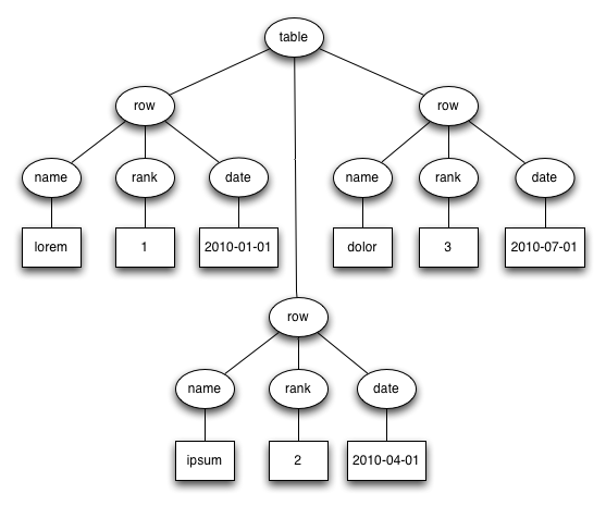
An arborescence is a connected, directed graph in which each node has at most one parent but can have multiple children. Edges point from parent to child. There is a unique node called the root which has no parent. Nodes with no children are called leaf nodes.
A tree is an arborescence in which the order of the children of each node is significant. In the examples above, the XML and the Lisp notation faithfully represent the tree. The JSON does not because the following two lines of JSON represent the same data:
{"foo":1, "bar:2}
{"bar":2, "foo"1}
Data which can be organized in trees or arborescences is hierarchical data. Hierarchical data can be constrained by restricting the types of data that can be the children of a given type of node. One formalism for specifying such restrictions is Backus-Naur Form (BNF), which was developed to specify the language Algol. Here is some BNF for the XML example above:
<table> ::= "<table>" {<row>} "</table>"
<row> ::= "<row>" <name> <rank> <date> "</row>"
<name> ::= "<name>" <any character except < and >> "</name>"
<rank> ::= "<rank>" <digits> "</rank>"
<date> ::= "<date>" 4 * <digit> "-" 2 * <digit> "-" 2 * <digit>" "</date>
No XML tree which satisfies the above rules will be deeper than three elements. BNF rulesets which employ recursion may place no bound on the depth of the trees which satisfy them. An example is the following BNF for algebraic expressions:
<expr> ::= <expr> "+" <term> | <expr> "-" <term> | <term>

<term> ::= <term> "*" <factor> | <term> "/" <factor> | <factor>

<factor> ::= <number> | "(" <expr> ")"
We've seen that hierarchical data formats can be used to represent data stored in tabular formats. If each node of data stored in a hierarchical format is assigned a unique identifier, then it is possible to represent hierarchical data in a tabular format:
| id | tag | text | parent id |
|---|---|---|---|
| 1 | table | <null> | <null> |
| 2 | row | <null> | 1 |
| 3 | row | <null> | 1 |
| 4 | row | <null> | 1 |
| 5 | name | lorem | 2 |
| 6 | rank | 1 | 2 |
| 7 | date | 2010-01-01 | 2 |
| 8 | name | ipsum | 3 |
| 9 | rank | 2 | 3 |
| 10 | date | 2010-04-01 | 3 |
| 11 | name | dolor | 4 |
| 12 | rank | 3 | 4 |
| 13 | date | 2010-07-01 | 4 |
An Aside on Serialization
Serialization is the conversion of a data structure to a string or stream of characters without loss of information.
XML, JSON, and Lisp notation are ways to serialize hierarchical data.
A common way to serialize tabular data is with field and record separators. Popular choices for the separators are tabs (ASCII 0x09) and newlines (ASCII 0x0A) respectively. When these characters occur in the data a strategy must be chosen for handling them. The ASCII standard designated the bytes 0x1C and 0x1E for use as a field separator and record separator. Perhaps because they are printable tabs and newlines are used more often.
Separators in the data can be handled in a variety of means. A simple measure is to strip them from the data. Another option is to substitute another character. For example it may be appropriate to replace tabs and newlines with a space character. Stripping and substitution mean that the data cannot be recovered in its original form, but they place the least demands on the program which must parse the data.
To preserve data that might contain the separators exactly as is, one can use escaping or quoting. In escaping, a character such as the backslash is designated as the escape character and special rules come into play when it is encountered. The escape character can be used before a separator to indicate that it is not be interpreted as a separator, or an escape sequences such as \t and \n can be used to represent the separator characters when they aren't being used as separators. If the escape character itself occurs in the data there must be a way of representing it, and duplication is the normal technique. That is, two backslashes \\ are used to represent a single backslash.
When quoting is used, the separators are not interpreted as such between and opening and closing quote character. The opening and closing quote characters may be the same such as ASCII double quotes "" or different such as parens (). The closing quote character must be escapable if it can appear in the data. An escape character can be introduced for use in strings, or duplication can be used to represent the closing quote character in the string.
Some programs may use field and record terminators instead of separators.
Search
Relational Algebra
A k-ary relation is a set of k-tuples. Relational algebra is the study of operators on relations. Tables are not the same as relations, however, since rows might be repeated and the order of the rows might be significant. Nevertheless relational algebra is the branch of mathematics most often used in database theory.
| relational algebra | SQL | Pig | |
|---|---|---|---|
| union | union | union | |
| intersection | intersect | none | |
| difference | except | none | |
| π | projection | select | foreach generate |
| σ | selection | where | filter |
| ρ | rename | as | as |
| ⋈ | natural join | join on | |
| cartesian product | from | cross |
History
An Occidental Ambiguity
In English, the word table shares the following two senses: (1) a piece of furniture consisting of a smooth flat slab fixed on legs, and (2) a systematic arrangement of data usu. in rows and columns for ready reference. Data which is arranged in rows and columns usually fits nicely into a rectangle and rectangles are a common tabletop shape, so the two senses aren't completely unrelated. Most other languages don't use the same word for both senses, however.
Wikipedia claims without citing a reference that the second sense derives from a practice of medieval Italian bankers; they would spread a checkered cloth on a table to count money.
Italian and French have cognate versions of table which share these two senses. Other languages I checked don't. I summarized my findings in a "table" table:
| language | furniture | figure | data structure |
|---|---|---|---|
| English | kitchen table | multiplication table | database table |
| Italian | tavolo da cucina | moltiplicazione tavolo | tabella del database |
| French | (la) table de cuisine | table de multiplication | table de la base |
| Spanish | mesa de cocina | tabla de multiplicación | base de datos de la tabla |
| Portuguese | mesa de cozinha | tabuada de multiplicar | tabela de banco |
| German | (der) Küchentisch | Multiplikationstabelle | Datenbanktabelle |
| Russian | кухонный стол | таблица умножения | таблицы базы данных |
| Arabic | طاولة المطبخ | جدول الضرب | قاعدة بيانات الجدول |
| Japanese | キッチンのテーブル | 九九の表 | データベースのテーブル |
| Chinese | 廚房的桌子 | 乘法表 | 數據庫中的表 |
It's my understanding that the Italians use both tavolo and tabella to refer to tables as furniture. I'm not sure if there is any distinction in meaning.
A classical Roman would use mensa to refer to a table used for eating and tabula to refer to a writing tablet. Spaniards and Portuguese are thus more conservative than other Romance language speakers in their choice of word for a table as furniture. Roman writing tablets were a hinged pair of wooden panels with depressions for holding wax. Such wax tablets were also used by Greeks from the mid 8th century BCE (per Wikipedia, no citation).
Germans and Russians have borrowed either directly or indirectly from Italian to get their words for the figure and the data structure. For the furniture they use native words. Tisch is cognate with the Engish dish and ultimately derives from the Latin discus so it is not strictly speaking native, but it has been in the German language longer than Tabelle. The Russian word for table as furniture стол is suspiciously close to the English stool, German Stuhl. The word is attested in Old High German and Old Church Slavonic. Here is a tweet from a woman in Moscow calling one of the tables on this website a табличка.
The Arabic word for a table as furniture طاولة (taawula) is borrowed from the Italian tavolo. The word which corresponds to table in multiplication table and database table is the native word جدول (jadwal) which means creek or brook. The Arabs are thus using a different metaphor, perhaps the same one used in the computer science term data stream.
The Japanese apparently favor the English loan word テーブル for a table as furniture, though they have a native word taku and a Kanji for it: 卓. 表 is pronounced hyo and is only used for a table as a figure.
Note that the Chinese character for the table furniture 桌 has two more strokes than the Japanese version. Another possible translation for it is desk. The pinyin is zhuo and it has a high tone. The pinyin for 表 is biao and it has a dip tone. Another possible translation is list.
Punch Cards
Punched Card Tabulating Machines Early Office Museum
Herman Hollerith won a contract from the US Census Bureau to process the 1890 US Census with punch cards. Hollerith designed a keypunch to encode census data on the cards. The keypunch used a pantograph for precision. To process the cards Hollerith designed a card reader which could be used for both counting and sorting. When used for counting the reader worked by completing an electrical circuit when the card had a hole in the right place. A hand on a dial with a hundred positions would advance. The dials had two hands like a clock so that together they could represent 10,000 values. The completion of an electrical circuit was also used when sorting. In this case the circuit completion would cause one of 24 lids to open, determining where the card ended up. Cards were fed into the reader manually one at a time.
The card reader that Hollerith built in 1890 could only be used for the 1890 census, but in 1906 Hollerith's company developed a general purpose tabulator that was programmable by means of a plugboard and patch cables which were called a control panel. Control panels were used to program two early computers: the Colossus used at Bletchley Park and the ENIAC. The phrase control panel lives on in the Windows operating system. The 1906 tabulator had an automatic card feed.
Hollerith's company was absorbed into the CTR Corporation in 1911. The company developed a printing tabulator in 1920. Previously numbers had to be read off of dials and recorded manually. The CTR Corporation renamed itself IBM in 1924. The company introduced a tabulator which could subtract in 1928. It also replaced the 45 column cards used since the 1890 census with the 80 column card that would be standard to the end of the punch card era.
In 1931 IBM introduced a tabulator which could multiply. In 1934 IBM introduced a fully alphabetic accounting machine. The machine could apparently print out reports with letters, not just numbers. I assume that letters could be stored on the punchcards as well. Was the encoding mechanism the same as the BCD 6-bit used for characters on the IBM 704 in 1954?
IBM punch card technology reached a high point with the IBM 407 introduced in 1949 and available as late as 1976. With it, a stack of punch cards, and accompanying machines one could perform many of the operations that one can perform on a database table today. Tabulators and accounting machines provided the aggregation functions COUNT and SUM. Sorting machines could implement GROUP BY. They could also implement ORDER BY by repeated application of radix sort. There were card duplicating machines. If they could be configured to duplicate only some of the columns they would be implementing projection (i.e. SELECT).
Early Computer Databases
The Programmer as Navigator (pdf) Bachman 1973
The first hard disk was the IBM 350 which had storage capacity of 5 million 7-bit characters (6-bit characters plus checksum bit) and a data transfer rate of 8.8k 7-bit characters per second. Average seek time was 600ms, and the unit weighed a ton. The IBM 1301 introduced in 1961 could store up to 56 million 7-bit characters and had a data transfer rate of 90k 7-bit characters per second. Worst case seek time was 180ms. The seek time of hard disk was much better than previously available persistent data stores such as punch cards or the magnetic tape used by the UNIVAC I. Hard disks made a new type of data store possible in which a record could be looked up quickly without scanning the entire set of records.
Richard Canning estimated in 1973 that there were 1000 to 2000 database systems installed worldwide. The most widely used database management systems at the time were IDS (1965), IMS (1968), and TDMS (1969).
IDS was developed by General Electric for Weyerhauser. The project started in 1961 and was led by Charles Bachman, who described the system in a paper in 1965. IDS supported both primary and secondary indices, the latter being distinguished by the fact that a lookup could yield more than one record. IDS also supported concurrent access by automatically rolling back and restarting transactions to resolve conflicts. Weyerhauser found that in typical usage about 10% of transactions were rolled back. IDS became a Honeywell product in 1970 when Honeywell acquired the GE computer division.
IMS was developed by IBM for the Apollo space program. It ran on System/360 and was available by 1968. IMS only supported a single index per table, and as a result it was less flexible than IDS in terms of the data that it could model and the lookup methods it could supprt. Joins between the dependent table and the parent table could be implemented in a language which was likely COBOL by scanning the child table and doing index lookups on the primary key of the parent.
TDMS (Time-shared Data Management System) was built by SDC (System Development Corporation), a division of RAND that was spun off as a separate organization in 1957. SDC did work for the military, especially the USAF. It designed one of the first time-sharing operating systems; the OS ran on the one-off AN/FSQ-32 mainframe used by ARPA. SDC developed the JOVIAL language, a dialect of ALGOL-58 used by USAF for its embedded systems. TDMS was used by the military before 1969; in 1969 SDC became a for-profit company and began to offer its software to other clients. An interesting feature of TDMS is that it always indexed all of the columns of its tables.
Relational Database Theory
A Relational Model of Data for Large Shared Data Banks (pdf) Codd 1970
Edgar Codd introduced the relational model for databases with a series of papers starting in 1970. He was only aware of one previous paper on the use of mathematical relations in describing databases. The hierarchical and network models are sometimes collectively called navigational models because they store pointers to other tables in columns. The relational model emphasizes joining on values instead of pointer. The join column does not have to contain the offsets or a primary keys of another table, and it may be possible to meaningfully join the column against more than one table.
Codd's criticism of the navigational models was that they exposed extraneous information to the application developer regarding how the data was stored, and this resulted in application code that tended to break when maintenance was performed on the database to improve performance or support new features.
Relational Database Implementation
SEQUEL: A Structured English Query Language ACM 1974
A History and Evaluation of System R ACM 1981
The 1995 SQL Reunion: People, Projects, and Politics
Codd had a difficult time convincing people inside of IBM of the importance of his ideas, or even getting people to understand them. In 1971 he proposed a query language called DSL/Alpha which used single characters for operators in a style reminiscent of APL. He managed to assemble a small team within IBM to work on a project called Gamma-0 which had something to do with relational databases.
Codd worked out of IBM's San Jose office, and his ideas spread to UC Berkeley, where the Ingres project and the QUEL query language got their start with a grant to build a "geo-query database system". A system which provided a prompt for entering queries was up and running by 1975.
Within IBM Donald Chamberlin, apparently not working closely with Codd but aware of his ideas, developed a relational database querying language called SQUARE sometime before he was transferred to the San Jose office in 1973. Chamberlin did not think that the mathematical notation favored by Codd would ever be popular. SQUARE apparently still used subscripts which Chamberlin discovered are inconvenient because they can't be typed.
IBM began work on a relational database system called System R in 1974. A new language called SEQUEL was developed that would be renamed SQL because a British aircraft company owned a trademark on SEQUEL. SEQUEL drew many ideas from SQUARE but it discarded subscripts and it also introduced a GROUP BY operator. The initial prototype for System R was a single user system which provided the user with a prompt for entering SQL statements.
The second prototype was a multi-user system with locking. It ran on System/370 hardware running either the VM/CMS or MVS/TSO operating systems. It supported embedding SQL in COBOL or PL/I. COBOL or PL/I source code containing SQL was precprocessed to replace the SQL with System/370 assembly code. The first external customer was Pratt & Whitney who had an installation up and running in 1977. There were internal customers and a few more external customers such as Upjohn and Boeing.
For some reason IBM discontinued work on System R and began work on SQL/DS to run on the DOS/VSE and VM/CMS operating systems and DB2 for MVS. In addition to company politics, factors coming into play might have been the operating systems and the underlying storage systems that needed to be supported as well as backward compatibility with IMS which was still popular with IBM customers.
DB2 was initially promised for 1979 but did not ship until 1983. A company that would rename itself Oracle in 1982 shipped a relational database product that supported SQL in 1979. Larry Ellison was aware of developments that were going on inside IBM as many of the results were published in papers. Ellison tried to make his product as compatible as possible with System R but IBM wouldn't share the error codes. Nevertheless Oracle became the leader; the features in the Oracle database defined the state of the art throughout the 1980s and 1990s.
The 1979 database was called version 2 though it was first version sold. It was written in assembly for the PDP-11. It could run on a VAX using a PDP-11 emulator. Oracle released version 3 in 1983. This version was a complete rewrite to C for portability and it enabled the company to support both VMS and Unix.
- Oracle v4 (1984): read consistency
- Oracle v5 (1985): separate client and server processes
- Oracle v6 (1988): row level locking, PL/SQL.
- Oracle v7 (1992): stored PL/SQL, triggers, referential integrity constraints.
In addition to IBM, Oracle competed against Informix and Sybase. Informix released a relational database for Unix in 1981 which used the QUEL language. In 1985 they released a version which supported SQL. Sybase entered the market with a relational database for Unix in 1987. Sybase contracted with Microsoft to build the SQL Server database which ran on OS/2 in 1989 and Windows NT in 1993. Starting with SQL Server 7 (1998) the code base was forked and Microsoft took over development of SQL Server.
Open Source Relational Databases
Although it isn't open source, mSQL is associated with the open source community because it runs on Linux and is available for free for non-commercial use. mSQL enjoyed a period of popularity from 1994 to 1997 when it was eclipsed by MySQL.
MySQL was released in 1995 by Swedish developers dissatisifed with mSQL. They founded a company called MySQL AB the same year. MySQL AB was sold to Sun Microsystems in 2008 which was in turn acquired by Oracle in 2010.
- MySQL 3.23 (2000): first open source version
- MySQL 4.1 (2004): subqueries, prepared statements
- MySQL 5.0 (2005): cursors, stored procedures, triggers
POSTGRES was a UC Berkeley project. The database was a successor to Ingres. Four versions were released between 1988 and 1993 that used the QUEL language. The source code was released under the MIT license, and two Berkeley grad students rewrote the database to support SQL and released the product as Postgres95. Development continued via a group of developers who collaborated over the internet.
- Postgres95 (1995)
- PostgreSQL 6.0 (1997): unique indexes
- PostgreSQL 6.1 (1997): multicolumn indexes, sequences
- PostgreSQL 6.2 (1997): triggers
- PostgreSQL 6.3 (1998): subselect
- PostgreSQL 6.4 (1998): PL/pgSQL
- PostgreSQL 7.0 (2000): foreign keys