Creating applications on Linux can be done using different ways, but there are a limited ways of doing, so using the simplest and the most functional programming languages and libraries, that’s why we’re going to have a quick look about creating applications under the Linux desktop using the GTK+ library with Python programming language which is called “PyGObject”.
PyGObject uses the GObject Introspection to create binding for programming languages like Python, PyGObject is the next generation from PyGTK, you can say that PyGObject = Python + GTK3.
Create GUI Applications in Linux – Part 1
Today, we’re going to start a series about creating GUI (Graphical User Interface) applications under the Linux desktop using GTK+ library and PyGobject language, the series will cover the following topics:
About Python
First of all, you must have some basic knowledge in Python; Python is a very modern and easy to use programming language. It’s one of the most famous programming languages in the world, using Python, you will be able to create many great applications & tools. You may take some free courses like those at codeacademy.com or you may read some books about Python at:
GTK+ is an open-source cross-platform toolkit to create graphical user interfaces for desktop applications, it was first started in 1998 as a GUI toolkit for the GIMP, later, it was used in many other applications and soon became one of the most famous libraries to create GUIs. GTK+ is released under the LGPL license.
Creating GUI Applications Under Linux
There are 2 ways for creating the applications using GTK+ & Python:
- Writing the graphical interface using code only.
- Designing the graphical interface using the “Glade” program; which is RAD tool to design GTK+ interfaces easily, Glade generates the GUI as a XML file which can be used with any programming language to build the GUI, after exporting the GUI’s XML file, we’ll be able to link the XML file with our program to do the jobs we want.
We’ll explain both ways in short.
The Code-Only Way
Writing the GUI using code only can be little bit hard for noob programmer’s and very time-wasting, but using it, we can create very functional GUIs for our programs, more than those we create using some tools like Glade.
Let’s take the following example.
#!/usr/bin/python
# -*- coding: utf-8 -*-

from gi.repository import Gtk

class ourwindow(Gtk.Window):

    def __init__(self):
        Gtk.Window.__init__(self, title="My Hello World Program")
        Gtk.Window.set_default_size(self, 400,325)
        Gtk.Window.set_position(self, Gtk.WindowPosition.CENTER)

        button1 = Gtk.Button("Hello, World!")
        button1.connect("clicked", self.whenbutton1_clicked)

        self.add(button1)

    def whenbutton1_clicked(self, button):
      print "Hello, World!"

window = ourwindow()
window.connect("delete-event", Gtk.main_quit)
window.show_all()
Gtk.main()
Copy the above code, paste it in a “test.py” file and set 755 permission on the test.py file and run the file later using “./test.py”, that’s what you will get.
# nano test.py
# chmod 755 test.py
# ./test.py
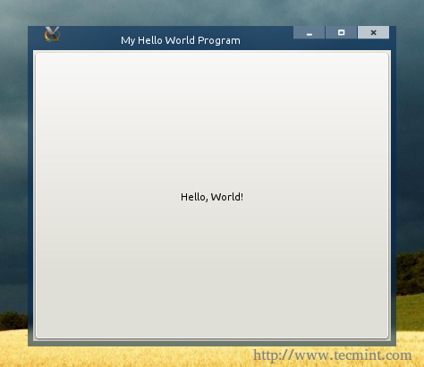
Hello World Script
By clicking the button, you see the “Hello, World!” sentence printed out in the terminal:
![]()
Test Python Script
Let me explain the code in detailed explanation.
- #!/usr/bin/python: The default path for the Python interpreter (version 2.7 in most cases), this line must be the first line in every Python file.
- # -*- coding: utf-8 -*-: Here we set the default coding for the file, UTF-8 is the best if you want to support non-English languages, leave it like that.
- from gi.repository import Gtk: Here we are importing the GTK 3 library to use it in our program.
- Class ourwindow(Gtk.Window): Here we are creating a new class, which is called “ourwindow”, we are also setting the class object type to a “Gtk.Window”.
- def __init__(self): Nothing new, we’re defining the main window components here.
- Gtk.Window.__init__(self, title=”My Hello World Program”): We’re using this line to set the “My Hello World Program” title to “ourwindow” window, you may change the title if you like.
- Gtk.Window.set_default_size(self, 400,325): I don’t think that this line need explanation, here we’re setting the default width and height for our window.
- Gtk.Window.set_position(self, Gtk.WindowPosition.CENTER): Using this line, we’ll be able to set the default position for the window, in this case, we set it to the center using the “Gtk.WindowPosition.CENTER” parameter, if you want, you can change it to “Gtk.WindowPosition.MOUSE” to open the window on the mouse pointer position.
- button1 = Gtk.Button(“Hello, World!”): We created a new Gtk.Button, and we called it “button1”, the default text for the button is “Hello, World!”, you may create any Gtk widget if you want.
- button1.connect(“clicked”, self.whenbutton1_clicked): Here we’re linking the “clicked” signal with the “whenbutton1_clicked” action, so that when the button is clicked, the “whenbutton1_clicked” action is activated.
- self.add(button1): If we want our Gtk widgets to appear, we have to add them to the default window, this simple line adds the “button1” widget to the window, it’s very necessary to do this.
- def whenbutton1_clicked(self, button): Now we’re defining the “whenbutton1_clicked” action here, we’re defining what’s going to happen when the “button1” widget is clicked, the “(self, button)” parameter is important in order to specific the signal parent object type.
- print “Hello, World!”: I don’t have to explain more here.
- window = ourwindow(): We have to create a new global variable and set it to ourwindow() class so that we can call it later using the GTK+ library.
- window.connect(“delete-event”, Gtk.main_quit): Now we’re connecting the “delete-event” signal with the “Gtk.main_quit” action, this is important in order to delete all the widgets after we close our program window automatically.
- window.show_all(): Showing the window.
- Gtk.main(): Running the Gtk library.
That’s it, easy isn’t? And very functional if we want to create some large applications. For more information about creating GTK+ interfaces using the code-only way, you may visit the official documentation website at:
The Glade Designer Way
Like I said in the beginning of the article, Glade is a very easy tool to create the interfaces we need for our programs, it’s very famous among developers and many great applications interfaces were created using it. This way is called “Rapid applications development”.
You have to install Glade in order to start using it, on Debian/Ubuntu/Mint run:
$ sudo apt-get install glade
On RedHat/Fedora/CentOS, run:
# yum install glade
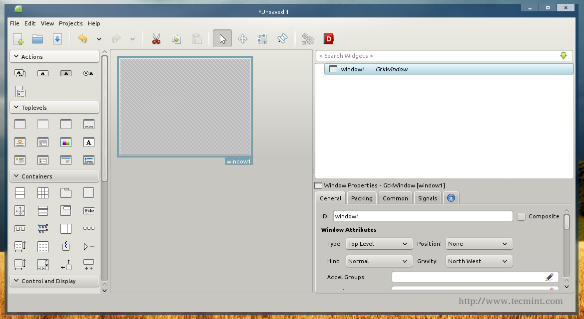
After you download and install the program, and after you run it, you will see the available Gtk widgets on the left, click on the “window” widget in order to create a new window.
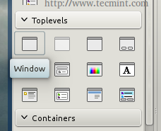
Create New Widget
You will notice that a new empty window is created.
New Window Widget
You can now add some widgets to it, on the left toolbar, click on the “button” widget, and click on the empty window in order to add the button to the window.
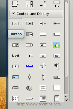
Add Widget
You will notice that the button ID is “button1”, now refer to the Signals tab in the right toolbar, and search for the “clicked” signal and enter “button1_clicked” under it.
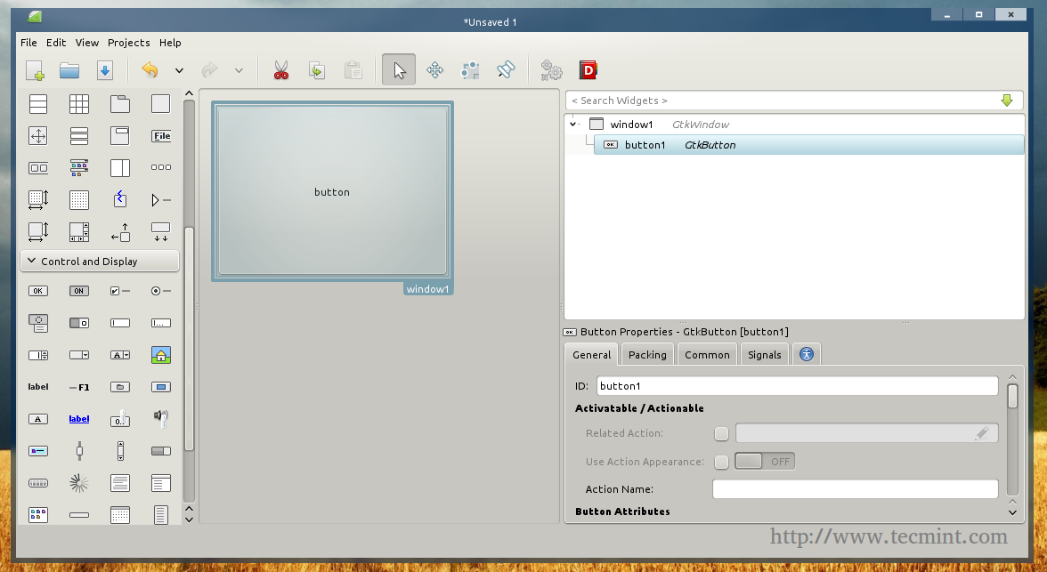
Button Properties
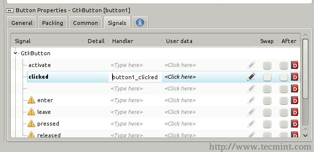
Signals Tab
Now that we’ve created our GUI, let’s export it. Click on the “File” menu and choose “Save”, save the file in your home directory in the name “myprogram.glade” and exit.
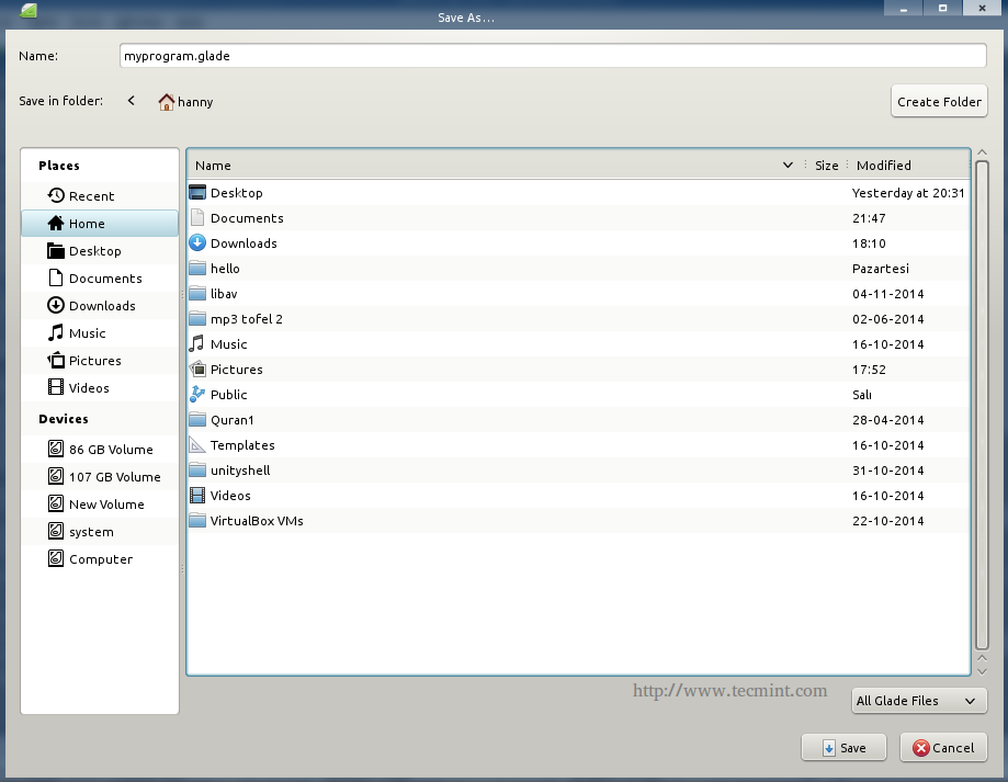
Export Widget File
Now, create a new “test.py” file, and enter the following code inside it.
#!/usr/bin/python
# -*- coding: utf-8 -*-

from gi.repository import Gtk

class Handler:
    def button_1clicked(self, button):
      print "Hello, World!"

builder = Gtk.Builder()
builder.add_from_file("myprogram.glade")
builder.connect_signals(Handler())

ournewbutton = builder.get_object("button1")
ournewbutton.set_label("Hello, World!")

window = builder.get_object("window1")

window.connect("delete-event", Gtk.main_quit)
window.show_all()
Gtk.main()
Save the file, give it 755 permissions like before, and run it using “./test.py”, and that’s what you will get.
# nano test.py
# chmod 755 test.py
# ./test.py

Hello World Window
Click on the button, and you will notice that the “Hello, World!” sentence is printed in the terminal.
Now let’s explain the new things:
- class Handler: Here we’re creating a class called “Handler” which will include the the definitions for the actions & signals, we create for the GUI.
- builder = Gtk.Builder(): We created a new global variable called “builder” which is a Gtk.Builder widget, this is important in order to import the .glade file.
- builder.add_from_file(“myprogram.glade”): Here we’re importing the “myprogram.glade” file to use it as a default GUI for our program.
- builder.connect_signals(Handler()): This line connects the .glade file with the handler class, so that the actions and signals that we define under the “Handler” class work fine when we run the program.
- ournewbutton = builder.get_object(“button1”): Now we’re importing the “button1” object from the .glade file, we’re also passing it to the global variable “ournewbutton” to use it later in our program.
- ournewbutton.set_label(“Hello, World!”): We used the “set.label” method to set the default button text to the “Hello, World!” sentence.
- window = builder.get_object(“window1”): Here we called the “window1” object from the .glade file in order to show it later in the program.
And that’s it! You have successfully created your first program under Linux!
Of course there are a lot more complicated things to do in order to create a real application that does something, that’s why I recommend you to take a look into the GTK+ documentation and GObject API at:
Have you developed any application before under the Linux desktop? What programming language and tools have used to do it? What do you think about creating applications using Python & GTK 3?
Create More Advance GUI Applications Using PyGobject Tool in Linux – Part 2
We continue our series about creating GUI applications under the Linux desktop using PyGObject, This is the second part of the series and today we’ll be talking about creating more functional applications using some advanced widgets.
Create Gui Applications in Linux- Part 2
Requirements
In the previous article we said that there are two ways for creating GUI applications using PyGObject: the code-only-way and the Glade designer way, but from now on, we’ll only be explaining the Glade designer way since it’s much easier for most users, you can learn the code-only-way by yourself using python-gtk3-tutorial.
Creating Advance GUI Applications in Linux
1. Let’s start programming! Open your Glade designer from the applications menu.
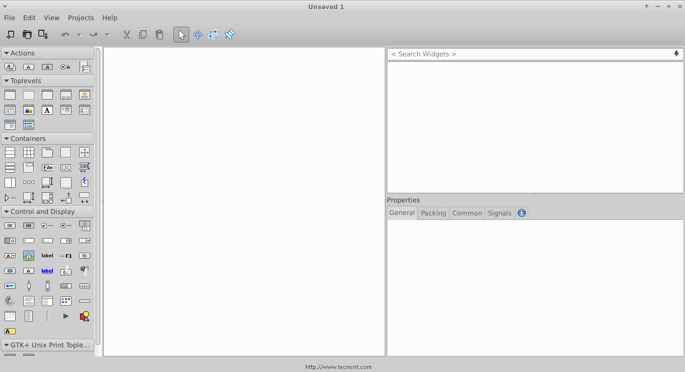
Glade Designer
2. Click on the “Window” button on the left sidebar in order to create a new one.
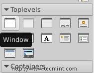
Create New Window
3. Click on the “Box” widget and release it on the empty window.
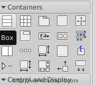
Select Box Widget
4. You will be prompted to enter the number of boxes you want, make it 3.
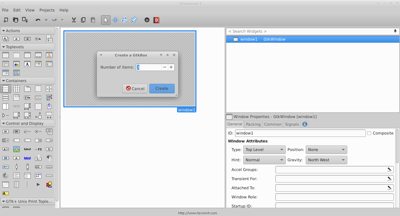
Create Boxes
And you’ll see that the boxes are created, those boxes are important for us in order to be able to add more than just 1 widget in a window.
5. Now click on the box widget, and change the orientation type from vertical to horizontal.
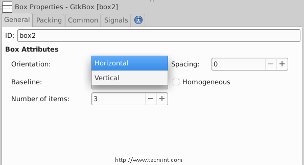
Make Box Horizontal
6. In order to create a simple program, add a “Text Entry”, “Combo Box Text” and a “Button” widgets for each one of the boxes, you should have something like this.
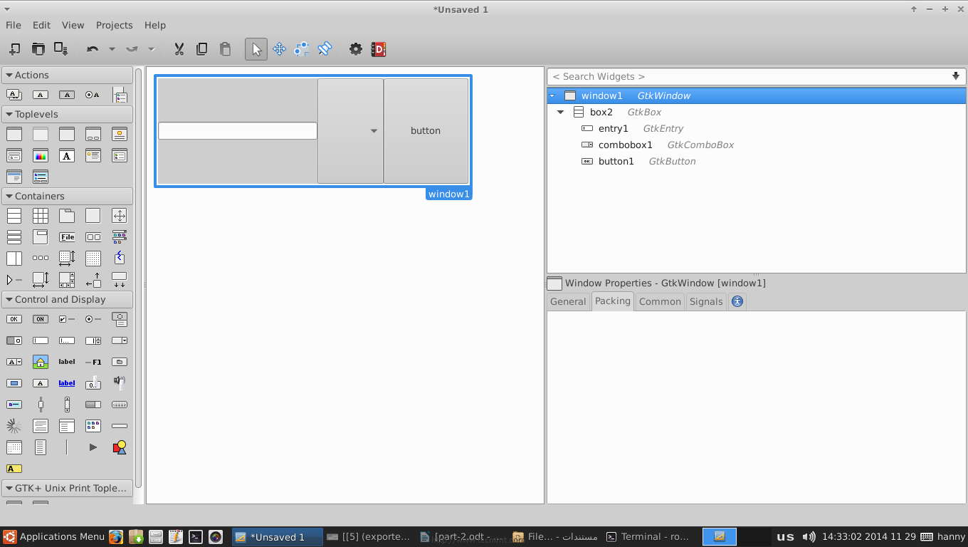
Create Simple Program
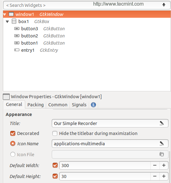
7. Now click on the “window1” widget from the right sidebar, and change its position to “Center“.
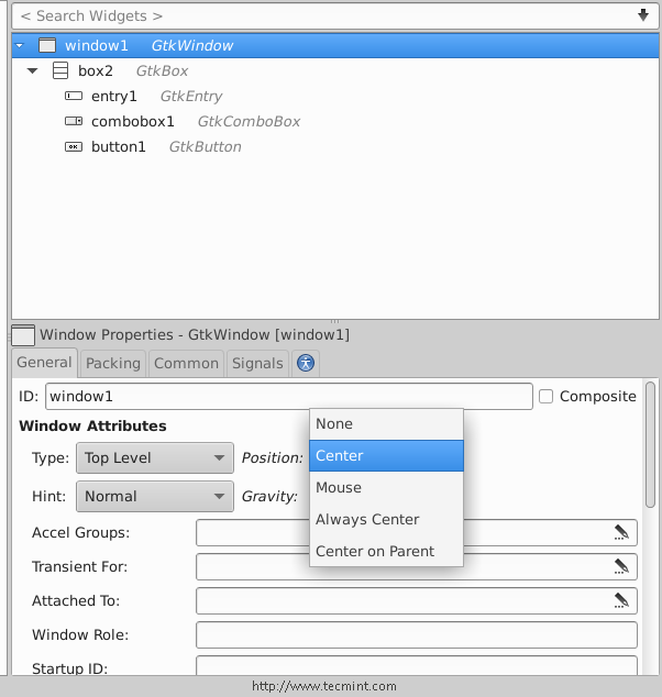
Make Widget Center
Scroll down to the “Appearance” section.. And add a title for the window “My Program“.
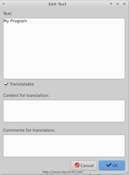
Add Widget Title
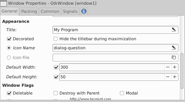
8. You can also choose an icon for the window by clicking on the “Icon Name” box.
![]()
Set Widget Icon
9. You can also change the default height & width for the application.. After all of that, you should have something like this.
Set Widget Height Width
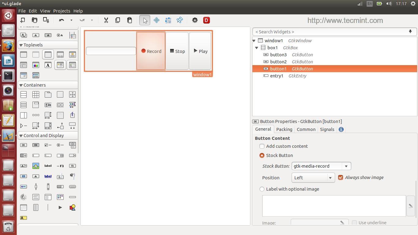
In any program, one of the most important thing is to create a “About” window, to do this, first we’ll have to change the normal button we created before into a stock button, look at the picture.
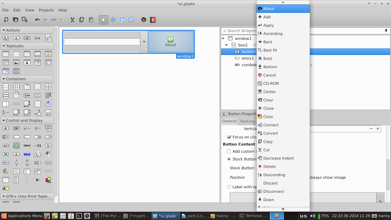
Create About Window
10. Now, we’ll have to modify some signals in order to run specific actions when any event occur on our widgets. Click on the text entry widget, switch to the “Signals” tab in the right sidebar, search for “activated” and change its handler to “enter_button_clicked”, the “activated” signal is the default signal that is sent when the “Enter” key is hit while focusing on the text entry widget.
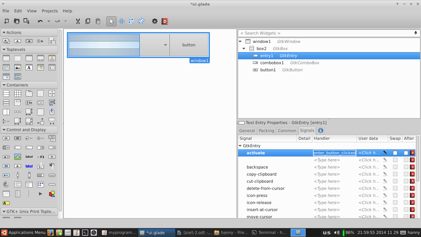
Set Widget Signals
We’ll have to add another handler for the “clicked” signal for our about button widget, click on it and change the “clicked” signal to “button_is_clicked“.
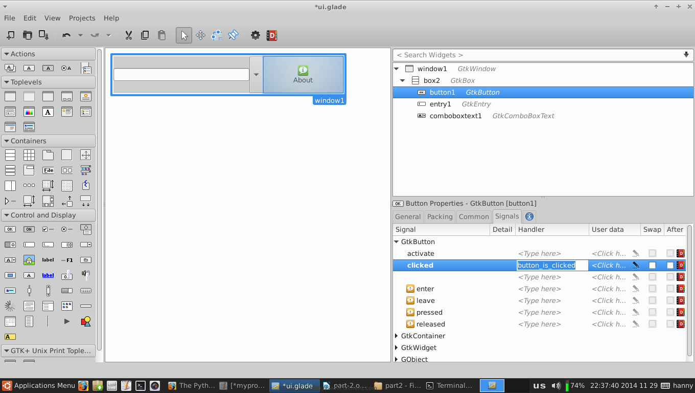
Add Widget Handler
11. Go to the “Common” tab and mark on “Has Focus” as it follows (To give the default focus for the about button instead of the entry).

Set Default Focus
12. Now from the left sidebar, create a new “About Dialog” window.
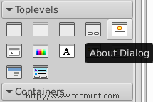
Create About Dialog
And you will notice that the “About Dialog” window is created.
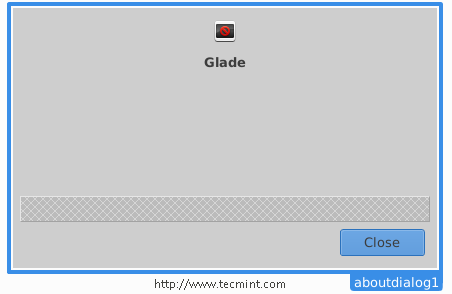
About Dialog
Let’s modify it.. Make sure that you insert the following settings for it from the right sidebar.
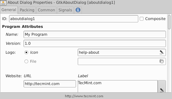
Add Program Attributes
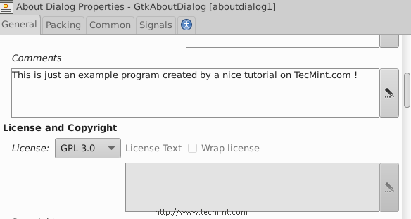
Select License
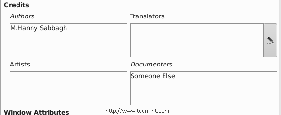
Add About Authors
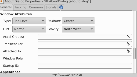
Set Window Appreance
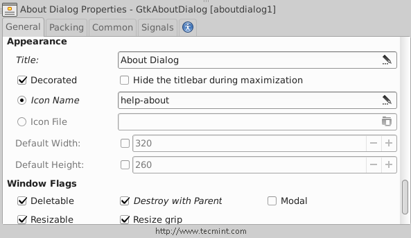
Select Appreance Flags
After making above settings, you will get following about Window.
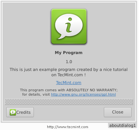
My Program about Window
In the above window, you will notice the empty space, but you can remove it by declining the number of boxes from 3 to 2 or you can add any widget to it if you want.
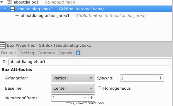
Change Window Boxes
13. Now save the file in your home folder in the name “ui.glade” and open a text editor and enter the following code inside it.
#!/usr/bin/python
# -*- coding: utf-8 -*-

from gi.repository import Gtk
class Handler:

    def button_is_clicked(self, button):
        ## The ".run()" method is used to launch the about window.
         ouraboutwindow.run()
        ## This is just a workaround to enable closing the about window.
         ouraboutwindow.hide()

    def enter_button_clicked(self, button):
        ## The ".get_text()" method is used to grab the text from the entry box. The "get_active_text()" method is used to get the selected item from the Combo Box Text widget, here, we merged both texts together".
         print ourentry.get_text() + ourcomboboxtext.get_active_text()

## Nothing new here.. We just imported the 'ui.glade' file.
builder = Gtk.Builder()
builder.add_from_file("ui.glade")
builder.connect_signals(Handler())

ournewbutton = builder.get_object("button1")

window = builder.get_object("window1")

## Here we imported the Combo Box widget in order to add some change on it.
ourcomboboxtext = builder.get_object("comboboxtext1")

## Here we defined a list called 'default_text' which will contain all the possible items in the Combo Box Text widget.
default_text = [" World ", " Earth ", " All "]

## This is a for loop that adds every single item of the 'default_text' list to the Combo Box Text widget using the '.append_text()' method.
for x in default_text:
  ourcomboboxtext.append_text(x)

## The '.set.active(n)' method is used to set the default item in the Combo Box Text widget, while n = the index of that item.
ourcomboboxtext.set_active(0)
ourentry = builder.get_object("entry1")

## This line doesn't need an explanation :D
ourentry.set_max_length(15)

## Nor this do.
ourentry.set_placeholder_text("Enter A Text Here..")

## We just imported the about window here to the 'ouraboutwindow' global variable.
ouraboutwindow = builder.get_object("aboutdialog1")

## Give that developer a cookie !
window.connect("delete-event", Gtk.main_quit)
window.show_all()
Gtk.main
Save the file in your home directory under that name “myprogram.py”, and give it the execute permission and run it.
$ chmod 755 myprogram.py
$ ./myprogram.py
This is what you will get, after running above script.
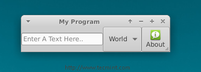
My Program Window
Enter a text in the entry box, hit the “Enter” key on the keyboard, and you will notice that the sentence is printed at the shell.
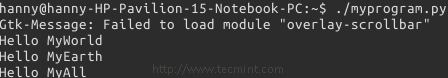
Box Output Text
That’s all for now, it’s not a complete application, but I just wanted to show you how to link things together using PyGObject, you can view all methods for all GTK widgets at gtkobjects.
Just learn the methods, create the widgets using Glade, and connect the signals using the Python file, That’s it! It’s not hard at all my friend.
We’ll explain more new things about PyGObject in the next parts of the series, till then stay updated and don’t forget to give us your comments about the article.
Create Your Own ‘Web Browser’ and ‘Desktop Recorder’ Applications Using PyGobject – Part 3
This is the 3rd part of the series about creating GUI applications under the Linux desktop using PyGObject. Today we’ll talk about using some advanced Python modules & libraries in our programs like ‘os‘, ‘WebKit‘, ‘requests‘ and others, beside some other useful information for programming.
Create Own Web Browser and Recorder – Part 3
Requirements
You must go through all these previous parts of the series from here, to continue further instructions on creating more advance applications:
- Create GUI Applications Under Linux Desktop Using PyGObject – Part 1
- Creating Advance PyGobject Applications on Linux – Part 2
Modules & libraries in Python are very useful, instead of writing many sub-programs to do some complicated jobs which will take a lot of time and work, you can just import them ! Yes, just import the modules & libraries you need to your program and you will be able to save a lot of time and effort to complete your program.
There are many famous modules for Python, which you can find at Python Module Index.
You can import libraries as well for your Python program, from “gi.repository import Gtk” this line imports the GTK library into the Python program, there are many other libraries like Gdk, WebKit.. etc.
Creating Advance GUI Applications
Today, we’ll create 2 programs:
- A simple web browser; which will use the WebKit library.
- A desktop recorder using the ‘avconv‘ command; which will use the ‘os’ module from Python.
I won’t explain how to drag & drop widgets in the Glade designer from now on, I will just tell you the name of the widgets that you need to create, additionally I will give you the .glade file for each program, and the Python file for sure.
Creating a Simple Web Browser
In order to create a web browser, we’ll have to use the “WebKit” engine, which is an open-source rendering engine for the web, it’s the same one which is used in Chrome/Chromium, for more info about it you may refer to the official Webkit.org website.
First, we’ll have to create the GUI, open the Glade designer and add the following widgets. For more information on how to create widgets, follow the Part 1 and Part 2 of this series (links given above).
- Create ‘window1’ widget.
- Create ‘box1’ and ‘box2’ widget.
- Create ‘button1’ and ‘button2’ widget.
- Create ‘entry1’ widget.
- Create ‘scrolledwindow1’ widget.
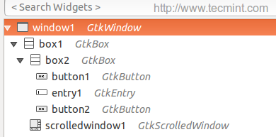
Add Widgets
After creating widgets, you will get the following interface.
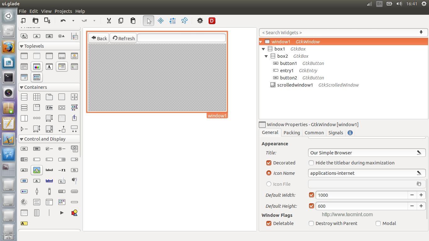
Glade Interface
There’s nothing new, except the “Scrolled Window” widget; this widget is important in order to allow the WebKitengine to be implanted inside it, using the “Scrolled Window” widget you will also be able to scroll horizontally and vertically while you browse the websites.
You will have now to add “backbutton_clicked” handler to the Back button “clicked” signal, “refreshbutton_clicked” handler to the Refresh button “clicked signal” and “enterkey_clicked” handler to the “activated” signal for the entry.
The complete .glade file for the interface is here.
<?xml version="1.0" encoding="UTF-8"?>
<!-- Generated with glade 3.16.1 -->
<interface>
  <requires lib="gtk+" version="3.10"/>
  <object class="GtkWindow" id="window1">
    <property name="can_focus">False</property>
    <property name="title" translatable="yes">Our Simple Browser</property>
    <property name="window_position">center</property>
    <property name="default_width">1000</property>
    <property name="default_height">600</property>
    <property name="icon_name">applications-internet</property>
    <child>
      <object class="GtkBox" id="box1">
        <property name="visible">True</property>
        <property name="can_focus">False</property>
        <property name="orientation">vertical</property>
        <child>
          <object class="GtkBox" id="box2">
            <property name="visible">True</property>
            <property name="can_focus">False</property>
            <child>
              <object class="GtkButton" id="button1">
                <property name="label">gtk-go-back</property>
                <property name="visible">True</property>
                <property name="can_focus">True</property>
                <property name="receives_default">True</property>
                <property name="relief">half</property>
                <property name="use_stock">True</property>
                <property name="always_show_image">True</property>
                <signal name="clicked" handler="backbutton_clicked" swapped="no"/>
              </object>
              <packing>
                <property name="expand">False</property>
                <property name="fill">True</property>
                <property name="position">0</property>
              </packing>
            </child>
            <child>
              <object class="GtkButton" id="button2">
                <property name="label">gtk-refresh</property>
                <property name="visible">True</property>
                <property name="can_focus">True</property>
                <property name="receives_default">True</property>
                <property name="relief">half</property>
                <property name="use_stock">True</property>
                <property name="always_show_image">True</property>
                <signal name="clicked" handler="refreshbutton_clicked" swapped="no"/>
              </object>
              <packing>
                <property name="expand">False</property>
                <property name="fill">True</property>
                <property name="position">1</property>
              </packing>
            </child>
            <child>
              <object class="GtkEntry" id="entry1">
                <property name="visible">True</property>
                <property name="can_focus">True</property>
                <signal name="activate" handler="enterkey_clicked" swapped="no"/>
              </object>
              <packing>
                <property name="expand">True</property>
                <property name="fill">True</property>
                <property name="position">2</property>
              </packing>
            </child>
          </object>
          <packing>
            <property name="expand">False</property>
            <property name="fill">True</property>
            <property name="position">0</property>
          </packing>
        </child>
        <child>
          <object class="GtkScrolledWindow" id="scrolledwindow1">
            <property name="visible">True</property>
            <property name="can_focus">True</property>
            <property name="hscrollbar_policy">always</property>
            <property name="shadow_type">in</property>
            <child>
              <placeholder/>
            </child>
          </object>
          <packing>
            <property name="expand">True</property>
            <property name="fill">True</property>
            <property name="position">1</property>
          </packing>
        </child>
      </object>
    </child>
  </object>
</interface>
Now copy the above code and paste it in the “ui.glade” file in your home folder. Now create a new file called “mywebbrowser.py” and enter the following code inside it, all the explanation is in the comments.
#!/usr/bin/python
# -*- coding: utf-8 -*-

## Here we imported both Gtk library and the WebKit engine.
from gi.repository import Gtk, WebKit

class Handler:

  def backbutton_clicked(self, button):
  ## When the user clicks on the Back button, the '.go_back()' method is activated, which will send the user to the previous page automatically, this method is part from the WebKit engine.
    browserholder.go_back()

  def refreshbutton_clicked(self, button):
  ## Same thing here, the '.reload()' method is activated when the 'Refresh' button is clicked.
    browserholder.reload()

  def enterkey_clicked(self, button):
  ## To load the URL automatically when the "Enter" key is hit from the keyboard while focusing on the entry box, we have to use the '.load_uri()' method and grab the URL from the entry box.
    browserholder.load_uri(urlentry.get_text())

## Nothing new here.. We just imported the 'ui.glade' file.
builder = Gtk.Builder()
builder.add_from_file("ui.glade")
builder.connect_signals(Handler())

window = builder.get_object("window1")

## Here's the new part.. We created a global object called 'browserholder' which will contain the WebKit rendering engine, and we set it to 'WebKit.WebView()' which is the default thing to do if you want to add a WebKit engine to your program.
browserholder = WebKit.WebView()

## To disallow editing the webpage.
browserholder.set_editable(False)

## The default URL to be loaded, we used the 'load_uri()' method.
browserholder.load_uri("https://tecmint.com")

urlentry = builder.get_object("entry1")
urlentry.set_text("https://tecmint.com")

## Here we imported the scrolledwindow1 object from the ui.glade file.
scrolled_window = builder.get_object("scrolledwindow1")

## We used the '.add()' method to add the 'browserholder' object to the scrolled window, which contains our WebKit browser.
scrolled_window.add(browserholder)

## And finally, we showed the 'browserholder' object using the '.show()' method.
browserholder.show()

## Give that developer a cookie !
window.connect("delete-event", Gtk.main_quit)
window.show_all()
Gtk.main()
Save the file, and run it.
$ chmod 755 mywebbrowser.py
$ ./mywebbrowser.py
And this is what you will get.
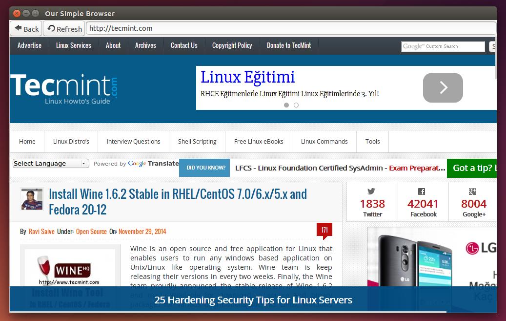
Create Own Web Browser
You may refer for the WebKitGtk official documentation in order to discover more options.
Creating a Simple Desktop Recorder
In this section, we’ll learn how to run local system commands or shell scripts from the Python file using the ‘os‘ module, which will help us to create a simple screen recorder for the desktop using the ‘avconv‘ command.
Open the Glade designer, and create the following widgets:
- Create ‘window1’ widget.
- Create ‘box1’ widget.
- Create ‘button1’, ‘button2’ and ‘button3’ widgets.
- Create ‘entry1’ widget.
Create Widgets
After creating above said widgets, you will get below interface.
Glade UI Interface
Here’s the complete ui.glade file.
<?xml version="1.0" encoding="UTF-8"?>
<!-- Generated with glade 3.16.1 -->
<interface>
  <requires lib="gtk+" version="3.10"/>
  <object class="GtkWindow" id="window1">
    <property name="can_focus">False</property>
    <property name="title" translatable="yes">Our Simple Recorder</property>
    <property name="window_position">center</property>
    <property name="default_width">300</property>
    <property name="default_height">30</property>
    <property name="icon_name">applications-multimedia</property>
    <child>
      <object class="GtkBox" id="box1">
        <property name="visible">True</property>
        <property name="can_focus">False</property>
        <child>
          <object class="GtkEntry" id="entry1">
            <property name="visible">True</property>
            <property name="can_focus">True</property>
          </object>
          <packing>
            <property name="expand">False</property>
            <property name="fill">True</property>
            <property name="position">0</property>
          </packing>
        </child>
        <child>
          <object class="GtkButton" id="button1">
            <property name="label">gtk-media-record</property>
            <property name="visible">True</property>
            <property name="can_focus">True</property>
            <property name="receives_default">True</property>
            <property name="use_stock">True</property>
            <property name="always_show_image">True</property>
            <signal name="clicked" handler="recordbutton" swapped="no"/>
          </object>
          <packing>
            <property name="expand">True</property>
            <property name="fill">True</property>
            <property name="position">1</property>
          </packing>
        </child>
        <child>
          <object class="GtkButton" id="button2">
            <property name="label">gtk-media-stop</property>
            <property name="visible">True</property>
            <property name="can_focus">True</property>
            <property name="receives_default">True</property>
            <property name="use_stock">True</property>
            <property name="always_show_image">True</property>
            <signal name="clicked" handler="stopbutton" swapped="no"/>
          </object>
          <packing>
            <property name="expand">True</property>
            <property name="fill">True</property>
            <property name="position">2</property>
          </packing>
        </child>
        <child>
          <object class="GtkButton" id="button3">
            <property name="label">gtk-media-play</property>
            <property name="visible">True</property>
            <property name="can_focus">True</property>
            <property name="receives_default">True</property>
            <property name="use_stock">True</property>
            <property name="always_show_image">True</property>
            <signal name="clicked" handler="playbutton" swapped="no"/>
          </object>
          <packing>
            <property name="expand">True</property>
            <property name="fill">True</property>
            <property name="position">3</property>
          </packing>
        </child>
      </object>
    </child>
  </object>
</interface>
As usual, copy the above code and paste it in the file “ui.glade” in your home directory, create a new “myrecorder.py” file and enter the following code inside it (Every new line is explained in the comments).
#!/usr/bin/python
# -*- coding: utf-8 -*-

## Here we imported both Gtk library and the os module.
from gi.repository import Gtk
import os

class Handler:
  def recordbutton(self, button):
    ## We defined a variable: 'filepathandname', we assigned the bash local variable '$HOME' to it + "/" + the file name from the text entry box.
    filepathandname = os.environ["HOME"] + "/" + entry.get_text()

    ## Here exported the 'filepathandname' variable from Python to the 'filename' variable in the shell.
    os.environ["filename"] = filepathandname

    ## Using 'os.system(COMMAND)' we can execute any shell command or shell script, here we executed the 'avconv' command to record the desktop video & audio.
    os.system("avconv -f x11grab -r 25 -s `xdpyinfo | grep 'dimensions:'|awk '{print $2}'` -i :0.0 -vcodec libx264 -threads 4 $filename -y & ")


  def stopbutton(self, button):
    ## Run the 'killall avconv' command when the stop button is clicked.
    os.system("killall avconv")

  def playbutton(self, button):
  ## Run the 'avplay' command in the shell to play the recorded file when the play button is clicked.
    os.system("avplay $filename &")


## Nothing new here.. We just imported the 'ui.glade' file.
builder = Gtk.Builder()
builder.add_from_file("ui.glade")
builder.connect_signals(Handler())

window = builder.get_object("window1")
entry = builder.get_object("entry1")
entry.set_text("myrecording-file.avi")

## Give that developer a cookie !
window.connect("delete-event", Gtk.main_quit)
window.show_all()
Gtk.main()
Now run the file by applying the following commands in the terminal.
$ chmod 755 myrecorder.py
$ ./myrecorder.py
And you got your first desktop recorder.
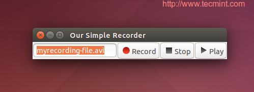
Create Desktop Recorder
You can find more information about the ‘os‘ module at Python OS Library.
And that’s it, creating applications for the Linux desktop isn’t hard using PyGObject, you just have to create the GUI, import some modules and link the Python file with the GUI, nothing more, nothing less. There are many useful tutorials about doing this in the PyGObject website:
Have you tried creating applications using PyGObject? What do you think about doing so? What applications have you developed before?
Package PyGObject Applications and Programs as “.deb” Package for the Linux Desktop – Part 4
We continue the PyGObject programming series with you on the Linux desktop, in the 4th part of the series we’ll explain how to package the programs and applications that we created for the Linux desktop using PyGObject as a Debian package.
Packaging Applications as Deb Package
Debian packages (.deb) are the most used format to install programs under Linux, the “dpkg” system which deals with .deb packages is the default on all Debian-based Linux distributions like Ubuntu and Linux Mint. That’s why we’ll be only explaining how to package our programs for Debian.
Create a Debian Package from your PyGObject Applications
First, you should have some basic knowledge about creating Debian packages, this following guide will help you a lot.
In brief, if you have project called “myprogram” it must contain the following files and folders so that you can package it.
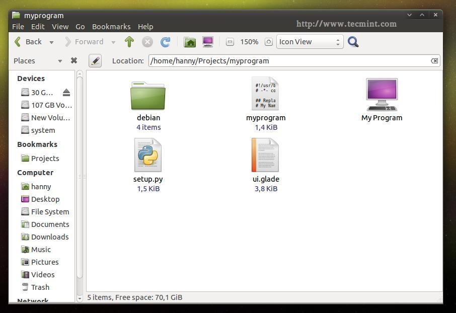
Create Deb Package
- debian (Folder): This folder includes all information about the Debian package divided to many sub-files.
- po (Folder): The po folder includes the translation files for the program (We’ll explain it in part 5).
- myprogram (File): This is the Python file we created using PyGObject, it’s the main file of the project.
- ui.glade (File): The graphical user interface file.. If you created the application’s interface using Glade, you must include this file in
your project. - bMyprogram.desktop (File): This is the responsible file for showing the application in the applications menu.
- setup.py (File): This file is the responsible for installing any Python program into the local system, it’s very important in any Python program, it has many other ways of usage as well.
Of course.. There are many other files and folders that you can include in your project (in fact you can include anything you want) but those are the basic ones.
Now, let’s start packaging a project. Create a new folder called “myprogram”, create a file called “myprogram” and add the following code to it.
#!/usr/bin/python
# -*- coding: utf-8 -*-

## Replace your name and email.
# My Name <myemail@email.com>

## Here you must add the license of the file, replace "MyProgram" with your program name.
# License:
#    MyProgram is free software: you can redistribute it and/or modify
#    it under the terms of the GNU General Public License as published by
#    the Free Software Foundation, either version 3 of the License, or
#    (at your option) any later version.
#
#    MyProgram is distributed in the hope that it will be useful,
#    but WITHOUT ANY WARRANTY; without even the implied warranty of
#    MERCHANTABILITY or FITNESS FOR A PARTICULAR PURPOSE.  See the
#    GNU General Public License for more details.
#
#    You should have received a copy of the GNU General Public License
#    along with MyProgram.  If not, see <http://www.gnu.org/licenses/>.

from gi.repository import Gtk
import os

class Handler:

  def openterminal(self, button):
    ## When the user clicks on the first button, the terminal will be opened.
    os.system("x-terminal-emulator ")

  def closeprogram(self, button):
    Gtk.main_quit()

# Nothing new here.. We just imported the 'ui.glade' file.
builder = Gtk.Builder()
builder.add_from_file("/usr/lib/myprogram/ui.glade")
builder.connect_signals(Handler())
window = builder.get_object("window1")
window.connect("delete-event", Gtk.main_quit)
window.show_all()
Gtk.main()
Create a ui.glade file and fill it up with this code.
<?xml version="1.0" encoding="UTF-8"?>
<!-- Generated with glade 3.16.1 -->
<interface>
  <requires lib="gtk+" version="3.10"/>
  <object class="GtkWindow" id="window1">
    <property name="can_focus">False</property>
    <property name="title" translatable="yes">My Program</property>
    <property name="window_position">center</property>
    <property name="icon_name">applications-utilities</property>
    <property name="gravity">center</property>
    <child>
      <object class="GtkBox" id="box1">
        <property name="visible">True</property>
        <property name="can_focus">False</property>
        <property name="margin_left">5</property>
        <property name="margin_right">5</property>
        <property name="margin_top">5</property>
        <property name="margin_bottom">5</property>
        <property name="orientation">vertical</property>
        <property name="homogeneous">True</property>
        <child>
          <object class="GtkLabel" id="label1">
            <property name="visible">True</property>
            <property name="can_focus">False</property>
            <property name="label" translatable="yes">Welcome to this Test Program !</property>
          </object>
          <packing>
            <property name="expand">False</property>
            <property name="fill">True</property>
            <property name="position">0</property>
          </packing>
        </child>
        <child>
          <object class="GtkButton" id="button2">
            <property name="label" translatable="yes">Click on me to open the Terminal</property>
            <property name="visible">True</property>
            <property name="can_focus">True</property>
            <property name="receives_default">True</property>
            <signal name="clicked" handler="openterminal" swapped="no"/>
          </object>
          <packing>
            <property name="expand">False</property>
            <property name="fill">True</property>
            <property name="position">1</property>
          </packing>
        </child>
        <child>
          <object class="GtkButton" id="button3">
            <property name="label">gtk-preferences</property>
            <property name="visible">True</property>
            <property name="can_focus">True</property>
            <property name="receives_default">True</property>
            <property name="use_stock">True</property>
          </object>
          <packing>
            <property name="expand">False</property>
            <property name="fill">True</property>
            <property name="position">2</property>
          </packing>
        </child>
        <child>
          <object class="GtkButton" id="button4">
            <property name="label">gtk-about</property>
            <property name="visible">True</property>
            <property name="can_focus">True</property>
            <property name="receives_default">True</property>
            <property name="use_stock">True</property>
          </object>
          <packing>
            <property name="expand">False</property>
            <property name="fill">True</property>
            <property name="position">3</property>
          </packing>
        </child>
        <child>
          <object class="GtkButton" id="button1">
            <property name="label">gtk-close</property>
            <property name="visible">True</property>
            <property name="can_focus">True</property>
            <property name="receives_default">True</property>
            <property name="use_stock">True</property>
            <signal name="clicked" handler="closeprogram" swapped="no"/>
          </object>
          <packing>
            <property name="expand">False</property>
            <property name="fill">True</property>
            <property name="position">4</property>
          </packing>
        </child>
      </object>
    </child>
  </object>
</interface>
There’s nothing new until now.. We just created a Python file and its interface file. Now create a “setup.py” file in the same folder, and add the following code to it, every line is explained in the comments.
# Here we imported the 'setup' module which allows us to install Python scripts to the local system beside performing some other tasks, you can find the documentation here: https://docs.python.org/2/distutils/apiref.html
from distutils.core import setup

setup(name = "myprogram", # Name of the program.
      version = "1.0", # Version of the program.
      description = "An easy-to-use web interface to create & share pastes easily", # You don't need any help here.
      author = "TecMint", # Nor here.
      author_email = "myemail@mail.com",# Nor here :D
      url = "http://example.com", # If you have a website for you program.. put it here.
      license='GPLv3', # The license of the program.
      scripts=['myprogram'], # This is the name of the main Python script file, in our case it's "myprogram", it's the file that we added under the "myprogram" folder.

# Here you can choose where do you want to install your files on the local system, the "myprogram" file will be automatically installed in its correct place later, so you have only to choose where do you want to install the optional files that you shape with the Python script
      data_files = [ ("lib/myprogram", ["ui.glade"]), # This is going to install the "ui.glade" file under the /usr/lib/myprogram path.
                     ("share/applications", ["myprogram.desktop"]) ] ) # And this is going to install the .desktop file under the /usr/share/applications folder, all the folder are automatically installed under the /usr folder in your root partition, you don't need to add "/usr/ to the path.
Now create a “myprogram.desktop” file in the same folder, and add the following code, it’s explained as well in the comments.
# This is the .desktop file, this file is the responsible file about showing your application in the applications menu in any desktop interface, it's important to add this file to your project, you can view more details about this file from here: https://developer.gnome.org/integration-guide/stable/desktop-files.html.en
[Desktop Entry]
# The default name of the program.
Name=My Program
# The name of the program in the Arabic language, this name will be used to display the application under the applications menu when the default language of the system is Arabic, use the languages codes to change the name for each language.
Name[ar]=برنامجي
# Description of the file.
Comment=A simple test program developed by me.
# Description of the file in Arabic.
Comment[ar]=برنامج تجريبي بسيط تم تطويره بواسطتي.
# The command that's going to be executed when the application is launched from the applications menu, you can enter the name of the Python script or the full path if you want like /usr/bin/myprogram
Exec=myprogram
# Do you want to run your program from the terminal?
Terminal=false
# Leave this like that.
Type=Application
# Enter the name of the icon you want to use for the application, you can enter a path for the icon as well like /usr/share/pixmaps/icon.png but make sure to include the icon.png file in your project folder first and in the setup.py file as well. Here we'll use the "system" icon for now.
Icon=system
# The category of the file, you can view the available categories from the freedesktop website.
Categories=GNOME;GTK;Utility;
StartupNotify=false
We’re almost done here now.. We just have to create some small files under the “debian” folder in order to provide information about our package for the “dpkg” system.
Open the “debian” folder, and create a the following files.
control
compat
changelog
rules
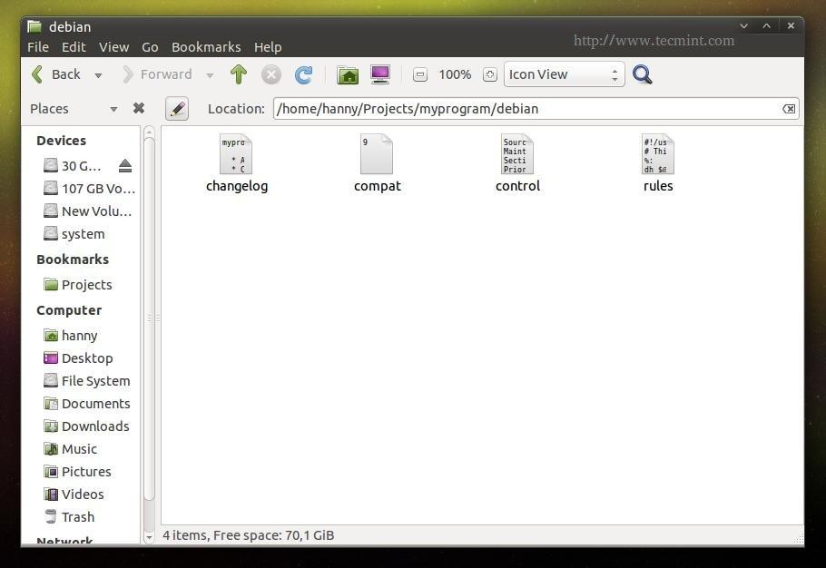
Project Files For Deb Package
control: This file provides the basic information about the Debian package, for more details, please visit Debian Package Control Fields.
Source: myprogram
Maintainer: My Name <myemail@email.com>
Section: utils
Priority: optional
Standards-Version: 3.9.2
Build-Depends: debhelper (>= 9), python2.7

Package: myprogram
Architecture: all
Depends: python-gi
Description: My Program
Here you can add a short description about your program.
compat: This is just an important file for the dpkg system, it just includes the magical 9 number, leave it like that.
9
changelog: Here you’ll be able to add the changes you do on your program, for more information, please visit Debian Package Changelog Source.
myprogram (1.0) trusty; urgency=medium

  * Add the new features here.
  * Continue adding new changes here.
  * And here.

 -- My Name Here <myemail@mail.com>  Sat, 27 Dec 2014 21:36:33 +0200
rules: This file is responsible about running the installation process on the local machine to install the package, you can view more information
about this file from here: Debian Package Default Rules.
Though you won’t need anything more for your Python program.
#!/usr/bin/make -f
# This file is responsible about running the installation process on the local machine to install the package, you can view more information about this file from here: https://www.debian.org/doc/manuals/maint-guide/dreq.en.html#defaultrules Though you won't need anything more for your Python program.
%:
    dh $@
override_dh_auto_install:
    python setup.py install --root=debian/myprogram --install-layout=deb --install-scripts=/usr/bin/ # This is going to run the setup.py file to install the program as a Python script on the system, it's also going to install the "myprogram" script under /usr/bin/ using the --install-scripts option, DON'T FORGET TO REPLACE "myprogram" WITH YOUR PROGRAM NAME.
override_dh_auto_build:
Now thats we created all the necessary files for our program successfully, now let’s start packaging it. First, make sure that you have installed some dependences for the build process before you start.
$ sudo apt-get update
$ sudo apt-get install devscripts
Now imagine that the “myprogram” folder is in your home folder (/home/user/myprogram) in order to package it as a Debian package, run the following commands.
$ cd /home/user/myprogram
$ debuild -us -uc
Sample Output
hanny@hanny-HP-Pavilion-15-Notebook-PC:~/Projects/myprogram$
debuild -us -uc dpkg-buildpackage -rfakeroot -D -us -uc
dpkg-buildpackage: source package myprogram
dpkg-buildpackage: source version 1.0
dpkg-buildpackage: source distribution trusty
dpkg-buildpackage: source changed by My Name Here
<myemail@email.com>
dpkg-source --before-build myprogram
dpkg-buildpackage: host architecture i386
fakeroot debian/rules clean
dh clean
dh_testdir
dh_auto_clean
....
.....
Finished running lintian.
And that’s it ! Your Debian package was created successfully:
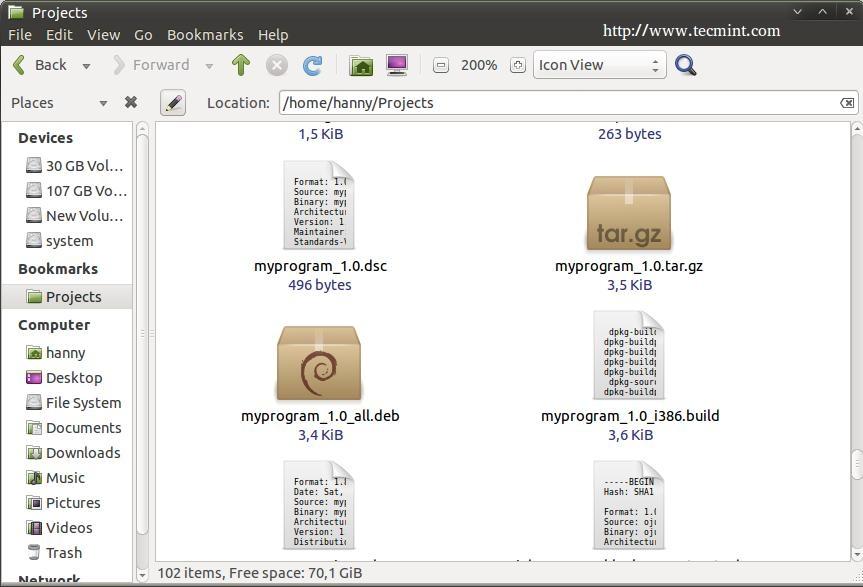
Created Debian Package
In order to install it on any Debian-based distribution, run.
$ sudo dpkg -i myprogram_1.0_all.deb
Don’t forget to replace the above file with the name of the package.. Now after you install the package, you can run the program from the applications menu.
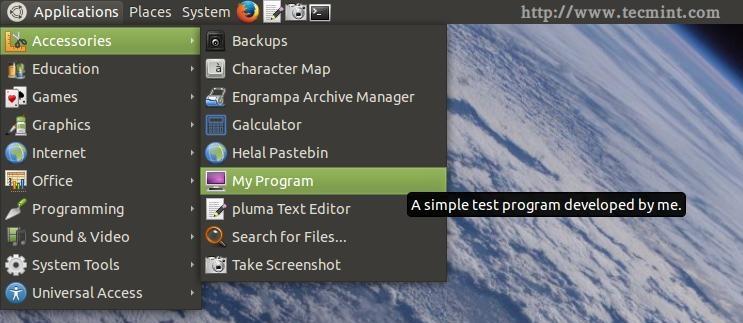
Run Program
And it will work..
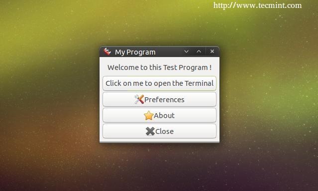
First Packaged Program
Here ends the 4th part of our series about PyGObject.. In the next lesson we’ll explain how to localize the PyGObject application easily, till then stay tunned for it…
Translating PyGObject Applications into Different Languages – Part 5
We continue the PyGObject programming series with you and here in this 5th part, we’ll learn how to translate our PyGObject applications into different languages. Translating your applications is important if you’re going to publish it for the world, it’ll be more user friendly for end-users because not everybody understands English.
Translating PyGObject Application Language
How the Translation Process Works
We can summarize the steps of translating any program under the Linux desktop using these steps:
- Extract the translatable strings from the Python file.
- Save the strings into a .pot file which is format that allows you to translate it later to other languages.
- Start translating the strings.
- Export the new translated strings into a .po file which will be automatically used when system language is changed.
- Add some small programmatic changes to the main Python file and the .desktop file.
And that’s it! After doing these steps your application will be ready for use for end-users from all around the globe (will.. You have to translate your program to all languages around the globe, though !), Sounds easy doesn’t it? 🙂
First, to save some time, download the project files from below link and extract the file in your home directory.
Open the “setup.py” file and notice the changes that we did:
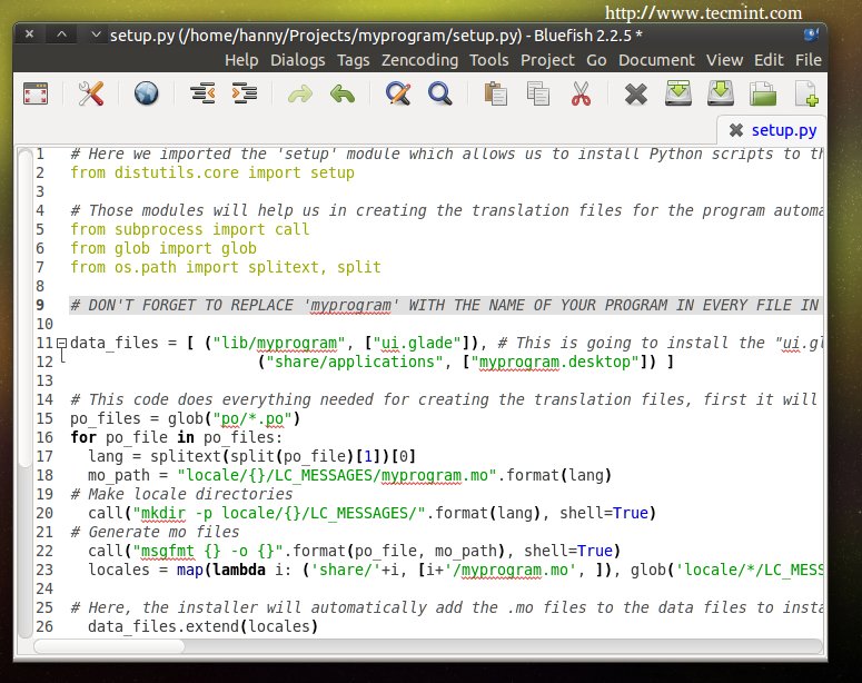
Translation Code
# Here we imported the 'setup' module which allows us to install Python scripts to the local system beside performing some other tasks, you can find the documentation here: https://docs.python.org/2/distutils/apiref.html
from distutils.core import setup

# Those modules will help us in creating the translation files for the program automatically.
from subprocess import call
from glob import glob
from os.path import splitext, split

# DON'T FOTGET TO REPLACE 'myprogram' WITH THE NAME OF YOUR PROGRAM IN EVERY FILE IN THIS PROJECT.

data_files = [ ("lib/myprogram", ["ui.glade"]), # This is going to install the "ui.glade" file under the /usr/lib/myprogram path.
                     ("share/applications", ["myprogram.desktop"]) ]

# This code does everything needed for creating the translation files, first it will look for all the .po files inside the po folder, then it will define the default path for where to install the translation files (.mo) on the local system, then it's going to create the directory on the local system for the translation files of our program and finally it's going to convert all the .po files into .mo files using the "msgfmt" command.
po_files = glob("po/*.po")
for po_file in po_files:
  lang = splitext(split(po_file)[1])[0]
  mo_path = "locale/{}/LC_MESSAGES/myprogram.mo".format(lang)
# Make locale directories
  call("mkdir -p locale/{}/LC_MESSAGES/".format(lang), shell=True)
# Generate mo files
  call("msgfmt {} -o {}".format(po_file, mo_path), shell=True)
  locales = map(lambda i: ('share/'+i, [i+'/myprogram.mo', ]), glob('locale/*/LC_MESSAGES'))

# Here, the installer will automatically add the .mo files to the data files to install them later.
  data_files.extend(locales)

setup(name = "myprogram", # Name of the program.
      version = "1.0", # Version of the program.
      description = "An easy-to-use web interface to create & share pastes easily", # You don't need any help here.
      author = "TecMint", # Nor here.
      author_email = "myemail@mail.com",# Nor here :D
      url = "http://example.com", # If you have a website for you program.. put it here.
      license='GPLv3', # The license of the program.
      scripts=['myprogram'], # This is the name of the main Python script file, in our case it's "myprogram", it's the file that we added under the "myprogram" folder.

# Here you can choose where do you want to install your files on the local system, the "myprogram" file will be automatically installed in its correct place later, so you have only to choose where do you want to install the optional files that you shape with the Python script
      data_files=data_files) # And this is going to install the .desktop file under the /usr/share/applications folder, all the folder are automatically installed under the /usr folder in your root partition, you don't need to add "/usr/ to the path.
Also open the “myprogram” file and see the programmatic changes that we did, all the changes are explained in the comments:
#!/usr/bin/python
# -*- coding: utf-8 -*-

## Replace your name and email.
# My Name <myemail@email.com>

## Here you must add the license of the file, replace "MyProgram" with your program name.
# License:
#    MyProgram is free software: you can redistribute it and/or modify
#    it under the terms of the GNU General Public License as published by
#    the Free Software Foundation, either version 3 of the License, or
#    (at your option) any later version.
#
#    MyProgram is distributed in the hope that it will be useful,
#    but WITHOUT ANY WARRANTY; without even the implied warranty of
#    MERCHANTABILITY or FITNESS FOR A PARTICULAR PURPOSE.  See the
#    GNU General Public License for more details.
#
#    You should have received a copy of the GNU General Public License
#    along with MyProgram.  If not, see <http://www.gnu.org/licenses/>.

from gi.repository import Gtk
import os, gettext, locale

## This is the programmatic change that you need to add to the Python file, just replace "myprogram" with the name of your program. The "locale" and "gettext" modules will take care about the rest of the operation.
locale.setlocale(locale.LC_ALL, '')
gettext.bindtextdomain('myprogram', '/usr/share/locale')
gettext.textdomain('myprogram')
_ = gettext.gettext
gettext.install("myprogram", "/usr/share/locale")

class Handler:

  def openterminal(self, button):
    ## When the user clicks on the first button, the terminal will be opened.
    os.system("x-terminal-emulator ")

  def closeprogram(self, button):
    Gtk.main_quit()

# Nothing new here.. We just imported the 'ui.glade' file.
builder = Gtk.Builder()
builder.add_from_file("/usr/lib/myprogram/ui.glade")
builder.connect_signals(Handler())

label = builder.get_object("label1")
# Here's another small change, instead of setting the text to ("Welcome to my Test program!") we must add a "_" char before it in order to allow the responsible scripts about the translation process to recognize that it's a translatable string.
label.set_text(_("Welcome to my Test program !"))

button = builder.get_object("button2")
# And here's the same thing.. You must do this for all the texts in your program, elsewhere, they won't be translated.
button.set_label(_("Click on me to open the Terminal"))


window = builder.get_object("window1")
window.connect("delete-event", Gtk.main_quit)
window.show_all()
Gtk.main()
Now.. Let’s start translating our program. First create the .pot file (a file that contains all the translatable strings in the program) so that you
can start translating using the following command:
$ cd myprogram
$ xgettext --language=Python --keyword=_ -o po/myprogram.pot myprogram
This is going to create the “myprogram.pot” file inside the “po” folder in the main project folder which contains the following code:
# SOME DESCRIPTIVE TITLE.
# Copyright (C) YEAR THE PACKAGE'S COPYRIGHT HOLDER
# This file is distributed under the same license as the PACKAGE package.
# FIRST AUTHOR <EMAIL@ADDRESS>, YEAR.
#
#, fuzzy
msgid ""
msgstr ""
"Project-Id-Version: PACKAGE VERSION\n"
"Report-Msgid-Bugs-To: \n"
"POT-Creation-Date: 2014-12-29 21:28+0200\n"
"PO-Revision-Date: YEAR-MO-DA HO:MI+ZONE\n"
"Last-Translator: FULL NAME <EMAIL@ADDRESS>\n"
"Language-Team: LANGUAGE <LL@li.org>\n"
"Language: \n"
"MIME-Version: 1.0\n"
"Content-Type: text/plain; charset=CHARSET\n"
"Content-Transfer-Encoding: 8bit\n"

#: myprogram:48
msgid "Welcome to my Test program !"
msgstr ""

#: myprogram:52
msgid "Click on me to open the Terminal"
msgstr ""
Now in order to start translating the strings.. Create a separated file for each language that you want to translate your program to using the “ISO-639-1” languages codes inside the “po” folder, for example, if you want to translate your program to Arabic, create a file called “ar.po” and copy the contents from the “myprogram.pot” file to it.
If you want to translate your program to German, create a “de.po” file and copy the contents from the “myprogram.pot” file to it.. and so one, you must create a file for each language that you want to translate your program to.
Now, we’ll work on the “ar.po” file, copy the contents from the “myprogram.pot” file and put it inside that file and edit the following:
- SOME DESCRIPTIVE TITLE: you can enter the title of your project here if you want.
- YEAR THE PACKAGE’S COPYRIGHT HOLDER: replace it with the year that you’ve created the project.
- PACKAGE: replace it with the name of the package.
- FIRST AUTHOR <EMAIL@ADDRESS>, YEAR: replace this with your real name, Email and the year that you translated the file.
- PACKAGE VERSION: replace it with the package version from the debian/control file.
- YEAR-MO-DA HO:MI+ZONE: doesn’t need explanation, you can change it to any date you want.
- FULL NAME <EMAIL@ADDRESS>: also replace it your your name and Email.
- Language-Team: replace it with the name of the language that you’re translating to, for example “Arabic” or “French”.
- Language: here, you must insert the ISO-639-1 code for the language that you’re translating to, for example “ar”, “fr”, “de”..etc, you can find a complete list here.
- CHARSET: this step is important, replace this string with “UTF-8” (without the quotes) which supports most languages.
Now start translating! Add your translation for each string after the quotes in “msgstr”. Save the file and exit. A good translation file for the
Arabic language as an example should look like this:
# My Program
# Copyright (C) 2014
# This file is distributed under the same license as the myprogram package.
# Hanny Helal <youremail@mail.com<, 2014.
#
#, fuzzy
msgid ""
msgstr ""
"Project-Id-Version: 1.0\n"
"Report-Msgid-Bugs-To: \n"
"POT-Creation-Date: 2014-12-29 21:28+0200\n"
"PO-Revision-Date: 2014-12-29 22:28+0200\n"
"Last-Translator: M.Hanny Sabbagh <hannysabbagh<@hotmail.com<\n"
"Language-Team: Arabic <LL@li.org<\n"
"Language: ar\n"
"MIME-Version: 1.0\n"
"Content-Type: text/plain; charset=UTF-8\n"
"Content-Transfer-Encoding: 8bit\n"

#: myprogram:48
msgid "Welcome to my Test program !"
msgstr "أهلًا بك إلى برنامجي الاختباري!"

#: myprogram:52
msgid "Click on me to open the Terminal"
msgstr "اضغط عليّ لفتح الطرفية"
There’s nothing more to do, just package the program using the following command:
$ debuild -us -uc
Now try to install the new created package using the following command.
$ sudo dpkg -i myprogram_1.0_all.deb
And change the system language using the “Language Support” program or using any other program to Arabic(or the language the you’ve translated your file to):
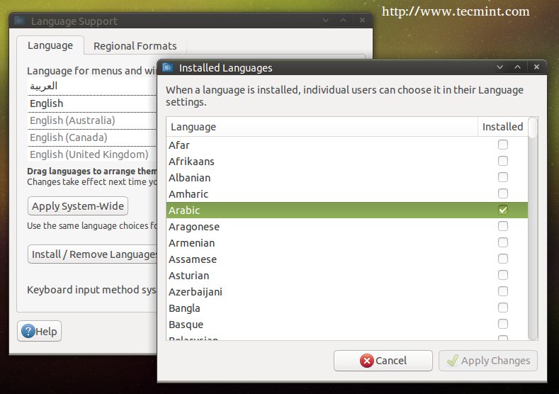
Language Support
After selecting, your program will be translated to Arabic language.
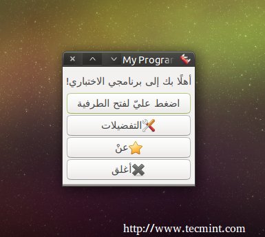
Translated to Arabic
Here ends our series about PyGObject programming for the Linux desktop, of course there are many other things that you can learn from the official documentation and the Python GI API reference..
What do you think about the series? Do you find it useful? Were you able to create your first application by following this series? Share us your thoughts!