Year: 2019

Linux news is getting more and more exciting, and somehow, managing to get less and less interesting. Why? Because the speed of development is getting so rapid that it’s hard to get excited for each upcoming release, keep your system completely up to date, and even remember what the current version of your favorite distributions are. This breakneck pace of development means good and bad things, but I have a few ideas about how I expect it to turn out.

The opinions in this piece are those of the author and not necessarily those of osnews.com

There are literally hundreds, if not thousands of distributions out there. In fact, with Knoppix, almost anyone can make his own. Each season, it seems we watch some distributions fold and others form. It’s getting harder and harder to tell them apart. Think you’re an expert? Answer these questions quickly:

5) Name three source-based distros.

According to a recent post on Distrowatch.com, “It is time to face the facts: the number of Linux distributions is growing at an alarming rate. On average, around 3 – 4 new distributions are submitted to this site every week, a fact that makes maintaining the individual pages and monitoring new releases increasingly time consuming. The DistroWatch database now lists a total of 205 Linux distributions (of which 24 have been officially discontinued) with 75 more on the waiting list. It is no longer easy to keep up.” Distributions change often, as does the popularity of each. Keeping up is almost impossible. Many Linux users install new distributions every few days, weeks, or months. Sadly, many of these folks keep a Windows installation – not because they prefer Windows, but because it’s a “safe haven” for their data which can’t find a permanent home on any given Linux distribution. Can this pace continue? I say no.

Predicting the future is always risky for an author, especially one who contributes to internet sites, where your words are often instantly accessible to the curious. But I’m going to put my money on the table and take some guesses about the future of Linux. Here, in no particular order, are six theories that I believe are inevitabilities. Keep in mind that although I’ve been liberal in tone, nearly everything in this piece is speculation or opinion and is subject to debate. Not all of these theories are necessarily entirely original thought, but all arguments are.

1) Major Linux distributions will collapse into a small, powerful group.
“Major players” in the Linux market, until recently, included Red Hat, SuSE, Mandrake, Debian, and Slackware. Some would argue more or less, but now you have a number of popular distros making inroads into the community, Xandros, LindowsOS, and Gentoo to name a few. Another fringe including Yoper, ELX, and TurboLinux are making plays for corporate desktops. I’m coining a new term for this era of Linux computing: distribution bloat. We have hundreds of groups offering us what is essentially minor tweaks and optimizations of a very similar base. This cannot continue at this pace. There will from this point on, be a growing number of Linux installation packages as people become more skilled, but there will be fewer distributions on a mass scale as commercial Linux stabilizes.

I think we’ll see the commercial Linux market boil down to two or three players, and this has already begun. I expect it to be a Ximian-ized Novell/SUSE distribution, Red Hat, and some sort of Debian offshoot – whether it’s User Linux or not remains to be seen. Sun’s Linux offering, Java Desktop System, will be deployed in Solaris committed companies and not much more.

2) Neither KDE nor Gnome will “win;” a third desktop environment will emerge.
The KDE/Gnome debate is a troll’s dream come true. People are often passionate about their desktop environment. I believe they both have strengths and weaknesses. However, a third DE, with a clean and usable base, will emerge in time, its sole mission to unify the Linux GUI. Only when there is true consistency of the look and feel of the desktop, or close to it, will Linux become a viable home OS for an average user. Currently, we see this consistency forged by common Qt and GKT themes, and offerings like Ximian Desktop which attempts to mask the different nature of each application. This is not about lack of choice – it is, however, about not allowing choice to supercede usability of the whole product.

Features that a desktop must include are obvious by now: cut & paste must work the same way throughout the OS, menus must be the same in all file manager windows, the same shortcut keys must apply in all applications, and all applications must have the same window borders. Many seemingly basic tasks that haven’t entirely matured, or in some cases, been accomplished at all, yet.

In any event, the DE’s importance will lessen once greater platform neutrality exists. This will doubtlessly cause many to argue that I am wrong – admittedly, it’s a tall order especially with Gnome and KDE becoming established and accomplishing so much. I maintain that unless there is some sort of merging, not a set of standards like freedesktop.org, but rather, a common base for development, that there will be a fragmented feel to Linux that simply doesn’t exist in Windows today.

3) Distribution optimization will become more prevalent
Most distributions today can be used for anything – a desktop system, a web server, a file server, a firewall, DNS, firewall, etc. I am of firm belief that Windows’ greater downfall on the server is that it has been a glorified desktop for too long. The file extensions are still hidden by default, you’re forced to run a GUI, and you can still run all your applications on the system. I predict that we’ll start to see flavors within distributions tweaked at the source level for optimization. Systems made to run as a desktop will have many different default options from their server optimized counterparts.

4) Integration will force the ultimate “killer app”
I predict an open, central authentication system will take the Linux world by storm. There still isn’t a Linux comparison to NDS/eDirectory or Active Directory that makes user management across the network as simple as either of the two. While eDirectory will run on Linux, there is no open standard with a GUI management tool that automates this mass management. An authentication service whose job is only to watch resources including users, devices, applications, and files doesn’t exist and can’t be built without serious Linux know-how. This service, which I’ll casually refer to as LCAS (Linux Central Authentication System) for lack of a better term, will be as easy to establish as a new Microsoft domain’s Active Directory.

LCAS will operate using completely open standards (X.500/LDAP) and will be easily ported to the BSDs and to commercial Unixes. Unlike Active Directory, LCAS services will be portable, and stored in a variety of databases, including PostgreSQL, MySQL, and even Oracle and DB2. LCAS, like Linux, will be pluggable, so that as it matures, management of other objects, like routers and switches, your firewall, and even workstations and PDAs and eventually, general network and local policies, will be controllable from your network LCAS installation. Perhaps, in time, it will also manage objects on the internet and how they can act within your network. I envision the ability to block, say, a particularly annoying application‘s HTTP traffic, the ability for certain users to use specified protocols, or installing internet printers via LCAS.

5) Releases will become less frequent, and updates more common
There is a competition for versioning in the Linux world, as though higher version numbers are somehow “better.” Version inflation is commonplace, with companies incrementing the major version for minor overall updates, and going from X.1 to (X+1) after a few application updates and a minor kernel increase. There is also a software trend that eventually, when the version number gets too high and is abandoned in favor of less harsh sounding names. No one would upgrade Windows every six months, so why upgrade Linux every six months? Because the software gets better too quickly! And the best way to get new software that works is to upgrade the whole distro! This is backward. The software should be incidental to the distro, not the reason for its version stamp.

Gentoo Linux just changed their release engineering guide specs to include for a year number with subsequent point releases. This, I think, is the right idea. I predict that we’ll start to see releases like DistroX 2004, DistroX 2005. As a counterpart, we’ll begin to see downloadable updates like service packs, like DistroX 2004 Update2. These updates will be easily installable and will update and patch not only the OS, but all components that came with the distro.

It is not unlikely that we’ll see a front end installer that launches, checks your system and the server, asks which pieces you want upgraded, and then processes it. There are systems like this in place today, however, they are constantly updated. Too often, people don’t patch or update, they just reinstall. We’re going to see only security updates for each distro, and approximately quarterly, we’ll see an official Update. Updates distributed in this fashion are much more likely to be applied by a common user than the slew of updates issued on an almost daily basis. Updates like this allow users to utilize a modern system much longer in between releases – for years in some cases. Unless OpenCarpet catches on, I see a service pack mentality prevailing for all commercial distributions.

6) Linux-approved hardware will become common
Part of the fight for useable Linux is with device drivers and hardware. Getting your video card to work properly, even with a binary driver available, is still way too hard. While this isn’t always the fault of the hardware, we will see, in time, Linux approved hardware. The hardware will include Linux drivers on the accompanying disk. There will be a certification process that tests hardware against a certain set of standards. Soon, a Tux badge on a PC case will be as commonplace as the “Built for Windows XX” stickers on most cases today.

I don’t claim to be visionary by any means. I also don’t want to forcefully bring spirituality into the mix, but I believe all things exist in waves, with highs and lows. Linux started small, it’s gained an audience, and as it swells to a large point, we, the community, should anticipate the future refold of things. The eventual downswing shouldn’t be an implosion, but rather, an opportunity to organize and streamline the existence of free software. It doesn’t have to be a reduction in use, it can be a simple cooperation, reduction of market saturation, and convergence towards standards.

Within the next two years, we’ll likely see Linux kernel 2.8, Gnome 3, and KDE 4. We’ll see exciting new projects. We’ll see many new Linux distributions and many existing ones disappear. We’ll see the pre-Microsoft Longhorn media blitz. And I bet, not too much longer than that, we’ll see some of the above start to become a reality as well.

Adam Scheinberg is a regular contributor to osnews.

Source

TurnKey Django Live CD is a free and open source software appliance, a special Debian-based operating system that has been designed from the ground up to provide users with an easy-to-use solution for deploying dedicated Django servers with minimum effort.

Django is an open source high-level Python web framework that promotes rapid application development, as well as pragmatic, clean design. The appliance comes with a pre-configured Django example project, which is installed by default in /var/www/project.

This Django project is integrated with the Apache web server using the mod_wsgi module, as well as with the MySQL database server and the Postfix mail server. In addition, it includes an administration console that features embedded online documentation.

Among other interesting components of this TurnKey appliance, we can mention the iPython command shell for interactive computing, Webmin modules for configuring the MySQL and Apache servers, as well as SSL for secure connections.

When installing this appliance, users should keep in mind that the default username for the Webmin, SSH and MySQL components is root, and that the default Django admin console username is admin. After installation, users will be able to enter new passwords for these accounts.

In order to have a fully functional Django server, you’ll also have to add a valid email address for the Django ‘admin’ account. Optionally, you can initialize the TurnKey Hub services for securely storing your files, databases and package management information.

The appliance is distributed as Live CD ISO images, allowing users to try it without installing anything on their computers. However, their main purpose is to install the operating system on a local disk drive. In addition to the Live CDs, the appliance is also available for download as virtual machine images for Xen, OVF, OpenNode, OpenVZ and OpenStack virtualization technologies.

TurnKey Linux Django LiveCD Operating system TurnKey Linux Django LiveCD

Source

In this lesson on Python Seaborn library, we will look at various aspects of this data visualisation library which we can use with Python to generate beautiful and intuitive graphs which can visualise data in a form which business wants from a platform. To make this lesson complete, we will cover the following sections:

• What is Python Seaborn?
• Types of Plots we can construct with Seaborn
• Working with Multiple plots
• Some alternatives for Python Seaborn

This looks like a lot to cover. Let us get started now.

What is Python Seaborn library?

Seaborn library is a Python package which allows us to make infographics based on statistical data. As it is made on top of matplotlib, so, it is inherently compatible with it. Additionally, it supports NumPy and Pandas data structure so that plotting can be done directly from those collections.

Visualising complex data is one of the most important thing Seaborn takes care of. If we were to compare Matplotlib to Seaborn, Seaborn is able to make those things easy which are hard to achieve with Matplotlib. However, it is important to note that Seaborn is not an alternative to Matplotlib but a complement of it. Throughout this lesson, we will make use of Matplotlib functions in the code snippets as well. You will select to work with Seaborn in the following use-cases:

• You have statistical time series data to be plotted with representation of uncertainty around the estimates
• To visually establish the difference between two subsets of data
• To visualise the univariate and bivariate distributions
• Adding much more visual affection to the matplotlib plots with many built-in themes
• To fit and visualise machine learning models through linear regression with independent and dependent variables

Just a note before starting is that we use a virtual environment for this lesson which we made with the following command:

Once the virtual environment is active, we can install Seaborn library within the virtual env so that examples we create next can be executed:

You can use Anaconda as well to run these examples which is easier. If you want to install it on your machine, look at the lesson which describes “How to Install Anaconda Python on Ubuntu 18.04 LTS” and share your feedback. Now, let us move forward to various types of plots which can be constructed with Python Seaborn.

To keep this lesson hands-on, We will use Pokemon dataset which can be downloaded from Kaggle. To import this dataset into our program, we will be using the Pandas library. Here are all the imports we perform in our program:

Now, we can import the dataset into our program and show some of the sample data with Pandas as:

Note that to run the above code snippet, the CSV dataset should be present in the same directory as the program itself. Once we run the above code snippet, we will see the following output (in Anaconda Jupyter’s notebook):

Plotting Linear Regression curve

One of the best thing about Seaborn is the intelligent plotting functions it provides which not only visualises the dataset we provide to it but also construct regression models around it. For example, it is possible to construct a linear regression plot with a single line of code. Here is how to do this:

Once we run the above code snippet, we will see the following output:

We noticed few important things in the above code snippet:

• There is dedicated plotting function available in Seaborn
• We used Seaborn’s fitting and plotting function which provided us with a linear regression line which it modelled itself

Don’t be afraid if you thought we cannot have a plot without that regression line. We can ! Let’s try a new code snippet now, similar to the last one:

This time, we will not see the regression line in our plot:

Now this is much more clear (if we do not need the linear regression line). But this isn’t just over yet. Seaborn allows us to make different this plot and that is what we will be doing.

Constructing Box Plots

One of the greatest feature in Seaborn is how it readily accepts Pandas Dataframes structure to plot data. We can simply pass a Dataframe to the Seaborn library so that it can construct a boxplot out of it:

Once we run the above code snippet, we will see the following output:

We can remove the first reading of total as that looks a little awkward when we are actually plotting individual columns here:

Once we run the above code snippet, we will see the following output:

Swarm Plot with Seaborn

We can construct an intuitive design Swarm plot with Seaborn. We will again be using the dataframe from Pandas which we loaded earlier but this time, we will be calling Matplotlib’s show function to show the plot we made. Here is the code snippet:

Once we run the above code snippet, we will see the following output:

By using a Seaborn context, we allow Seaborn to add a personal touch and fluid design for the plot. It is possible to customise this plot even further with custom font size used for labels in the plot to make the reading easier. To do this, we will be passing more parameters to the set_context function which performs just like what they sound. For example, to modify the font size of the labels, we will make use of font.size parameter. Here is the code snippet to do the modification:

Once we run the above code snippet, we will see the following output:

The font size for the label was changed based on the parameters we provided and value associated to the font.size parameter. One thing Seaborn is expert at is to make the plot very intuitive for practical usage and this means that Seaborn is not just a practice Python package but actually something we can use in our production deployments.

Adding a Title to plots

It is easy to add titles to our plots. We just need to follow a simple procedure of using the Axes-level functions where we will call the set_title() function like we show in the code snippet here:

Once we run the above code snippet, we will see the following output:

This way, we can add much more information to our plots.

Seaborn vs Matplotlib

As we looked at the examples in this lesson, we can identify that Matplotlib and Seaborn cannot be directly compared but they can be seen as complementing each other. One of the features which takes Seaborn 1 step ahead is the way Seaborn can visualise data statistically.

To make best of Seaborn parameters, we highly recommend to look at the Seaborn documentation and find out what parameters to use to make your plot as close to business needs as possible.

Conclusion

In this lesson, we looked at various aspects of this data visualisation library which we can use with Python to generate beautiful and intuitive graphs which can visualise data in a form which business wants from a platform. The Seaborm is one of the most important visualisation library when it comes to data engineering and presenting data in most visual forms, definitely a skill we need to have under our belt as it allows us to build linear regression models.

Source

Since receiving the powerful NVIDIA Jetson AGX Xavier with its ARMv8 Carmel cores on this Tegra194 SoC a while back, it’s been quite a fun developer board for benchmarking and various Linux tests. One of the areas I was curious about was whether GCC or Clang would generate faster code for this high performance ARM SoC, so here are some benchmarks.

This CPU compiler benchmarking was done with the NVIDIA Jetson AGX Xavier while running the Ubuntu 18.04 LTS default L4T file-system and comparing the default GCC 7.3.0 against LLVM Clang 6.0 compiler options as officially supported by Ubuntu LTS Bionic Beaver. These are also the compiler versions supported by NVIDIA with their Tegra software on this Linux 4 Tegra sample file-system. The NVIDIA Tegra Xavier (T194) SoC as a reminder has eight “Carmel” ARMv8 CPU cores that are custom designed by NVIDIA. Tests on other more common ARMv8 cores with these different compilers will be coming up in future Phoronix articles with Clang 8 and GCC 9 releasing later this quarter. Rounding out this powerful Jetson AGX Xavier is the Volta GPU with 512 CUDA cores, 16GB of LPDDR4 system memory, 32GB of eMMC storage, two NVDLA deep learning accelerators, and a 7-way vision processor, granted those aren’t the focus of today’s testing.

Via the Phoronix Test Suite a wide range of C/C++ benchmarks were carried out on this platform for seeing how the GCC and Clang compilers compare from Ubuntu 18.04 LTS.

Source

Securing your Linux server(s) is a difficult and time consuming task for System Administrators but its necessary to harden the server’s security to keep it safe from Attackers and Black Hat Hackers. You can secure your server by configuring the system properly and installing as minimum softwares as possible. There are some tips which can help you secure your server from network and privilege escalation attacks.

Upgrade your Kernel

Outdated kernel is always prone to several network and privilege escalation attacks. So you can update your kernel using apt in Debian or yum in Fedora.

Disabling Root Cron Jobs

Cron jobs running by root or high privilege account can be used as a way to gain high privileges by attackers. You can see running cron jobs by

Strict Firewall Rules

You should block any unnecessary inbound or outbound connection on uncommon ports. You can update your firewalls rules by using iptables. Iptables is a very flexible and easy to use utility used to block or allow incoming or outgoing traffic. To install, write

Here’s an example to block incoming on FTP port using iptables

Disable unnecessary Services

Stop any unwanted services and daemons running on your system. You can list running services using following commands.

OR using the following command

To stop a service, type

OR

Check for Backdoors and Rootkits

Utilities like rkhunter and chkrootkit can be used to detect known and unknown backdoors and rootkits. They verify installed packages and configurations to verify system’s security. To install write,

To scan your system, type

Check Listening Ports

You should check for listening ports that aren’t used and disable them. To check for open ports, write.

Use an IDS (Intrusion Testing System)

Use an IDS to check network logs and to prevent any malicious activities. There’s an open source IDS Snort available for Linux. You can install it by,

To monitor network traffic, type

Disable Logging as Root

Root acts as a user with full privileges, it has power to do anything with the system. Instead, you should enforce using sudo to run administrative commands.

Remove no owner Files

Files owned by no user or group can be security threat. You should search for these files and remove them or assign them a proper user a group. To search for these files, type

Use SSH and sFTP

For file transferring and remote administration, use SSH and sFTP instead of telnet and other insecure, open and unencrypted protocols. To install, type

Monitor Logs

Install and setup a log analyzer utility to check system logs and event data regularly to prevent any suspicious activity. Type

Uninstall unused Softwares

Install softwares as minimum as possible to maintain small attack surface. The more softwares you have, the more chances of attacks you have. So remove any unneeded software from your system. To see installed packages, write

To remove a package:

Conlusion

Linux server security hardening is very important for enterprises and businesses. Its a difficult and tiresome task for System Administrators. Some processes can be automated by some automated utilities like SELinux and other similar softwares. Also, keeping minimus softwares and disabling unused services and ports reduces the attack surface.

Source

Devstack is a collection of scripts which deploy the latest version of openstack environment on virtual machine, personal laptop or a desktop. As the name suggests it is used for development environment and can be used for Openstack Project’s functional testing and sometime openstack environment deployed by devstack can also be used for demonstrations purpose and for some basic PoC.

In this article I will demonstrate how to install Openstack on CentOS 7 / RHEL 7 System using Devstack. Following are the minimum system requirements,

• Dual Core Processor
• Minimum 8 GB RAM
• 60 GB Hard Disk
• Internet Connection

Following are  the details of my Lab Setup for Openstack deployment using devstack

• Minimal Installed CentOS 7 / RHEL 7 (VM)
• Hostname – devstack-linuxtechi
• IP Address – 169.144.104.230
• 10 vCPU
• 14 GB RAM
• 60 GB Hard disk

Let’s start deployment steps, login to your CentOS 7 or RHEL 7 System

Step:1 Update Your System and Set Hostname

Run the following yum command to apply latest updates to system and then take a reboot. Also after reboot set the hostname

~]# yum update -y && reboot
~]# hostnamectl set-hostname "devstack-linuxtechi"
~]# exec bash

Step:2) Create a Stack user and assign sudo rights to it

All the installations steps are to be carried out by a user name “stack“, refer the below commands to create and assign sudo rights .

[root@devstack-linuxtechi ~]# useradd -s /bin/bash -d /opt/stack -m stack
[root@devstack-linuxtechi ~]# echo "stack ALL=(ALL) NOPASSWD: ALL" | sudo tee /etc/sudoers.d/stack
stack ALL=(ALL) NOPASSWD: ALL
[root@devstack-linuxtechi ~]#

Step:3) Install git and download devstack

Switch to stack user and install git package using yum command

[root@devstack-linuxtechi ~]# su - stack
[stack@devstack-linuxtechi ~]$ sudo yum install git -y

Download devstack using below git command,

[stack@devstack-linuxtechi ~]$ git clone https://git.openstack.org/openstack-dev/devstack
Cloning into 'devstack'...
remote: Counting objects: 42729, done.
remote: Compressing objects: 100% (21438/21438), done.
remote: Total 42729 (delta 30283), reused 32549 (delta 20625)
Receiving objects: 100% (42729/42729), 8.93 MiB | 3.77 MiB/s, done.
Resolving deltas: 100% (30283/30283), done.
[stack@devstack-linuxtechi ~]$

Step:4) Create local.conf file and start openstack installation

To start openstack installation using devstack script (stack.sh), first we need to prepare local.conf file that suits to our setup.

Change to devstack folder and create local.conf file with below contents

[stack@devstack-linuxtechi ~]$ cd devstack/
[stack@devstack-linuxtechi devstack]$ vi local.conf
[[local|localrc]]
#Specify the IP Address of your VM / Server in front of HOST_IP Parameter
HOST_IP=169.144.104.230

#Specify the name of interface of your Server or VM in front of FLAT_INTERFACE
FLAT_INTERFACE=eth0

#Specify the Tenants Private Network and its Size
FIXED_RANGE=10.4.128.0/20
FIXED_NETWORK_SIZE=4096

#Specify the range of external IPs that will be used in Openstack for floating IPs
FLOATING_RANGE=172.24.10.0/24

#Number Host on which Openstack will be deployed
MULTI_HOST=1

#Installation Logs file
LOGFILE=/opt/stack/logs/stack.sh.log

#KeyStone Admin Password / Database / RabbitMQ / Service Password
ADMIN_PASSWORD=openstack
DATABASE_PASSWORD=db-secret
RABBIT_PASSWORD=rb-secret
SERVICE_PASSWORD=sr-secret

#Additionally installing Heat Service
enable_plugin heat https://git.openstack.org/openstack/heat master
enable_service h-eng h-api h-api-cfn h-api-cw

Save and exit the file.

Now start the deployment or installation by executing the script (stack.sh)

[stack@devstack-linuxtechi devstack]$ ./stack.sh

It will take between 30 to 45 minutes depending upon your internet connection.

While running the above command, if you got the below errors

+functions-common:git_timed:607            timeout -s SIGINT 0 git clone git://git.openstack.org/openstack/requirements.git /opt/stack/requirements --branch master
fatal: unable to connect to git.openstack.org:
git.openstack.org[0: 104.130.246.85]: errno=Connection timed out
git.openstack.org[1: 2001:4800:7819:103:be76:4eff:fe04:77e6]: errno=Network is unreachable
Cloning into '/opt/stack/requirements'...
+functions-common:git_timed:610            [[ 128 -ne 124 ]]
+functions-common:git_timed:611            die 611 'git call failed: [git clone' git://git.openstack.org/openstack/requirements.git /opt/stack/requirements --branch 'master]'
+functions-common:die:195                  local exitcode=0
[Call Trace]
./stack.sh:758:git_clone
/opt/stack/devstack/functions-common:547:git_timed
/opt/stack/devstack/functions-common:611:die
[ERROR] /opt/stack/devstack/functions-common:611 git call failed: [git clone git://git.openstack.org/openstack/requirements.git /opt/stack/requirements --branch master]
Error on exit
/bin/sh: brctl: command not found
[stack@devstack-linuxtechi devstack]$

To Resolve these errors, perform the following steps

Install bridge-utils package and change parameter from “GIT_BASE=${GIT_BASE:-git://git.openstack.org}” to “GIT_BASE=${GIT_BASE:-https://www.github.com}” in stackrc file

[stack@devstack-linuxtechi devstack]$ sudo yum install bridge-utils -y
[stack@devstack-linuxtechi devstack]$ vi stackrc
……
#GIT_BASE=${GIT_BASE:-git://git.openstack.org}
GIT_BASE=${GIT_BASE:-https://www.github.com}
……

Now re-run the stack.sh script,

[stack@devstack-linuxtechi devstack]$ ./stack.sh

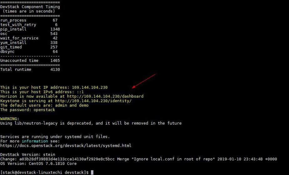
Once the script is executed successfully, we will get the output something like below,

This confirms that openstack has been deployed successfully,

Step:5 Access OpenStack either via Openstack CLI or Horizon Dashboard

if you want to perform any task from openstack cli, then you have to firsr source openrc file, which contain admin credentials.

[stack@devstack-linuxtechi devstack]$ source openrc
WARNING: setting legacy OS_TENANT_NAME to support cli tools.
[stack@devstack-linuxtechi devstack]$ openstack network list
+--------------------------------------+---------+----------------------------------------------------------------------------+
| ID                                   | Name    | Subnets                                                                    |
+--------------------------------------+---------+----------------------------------------------------------------------------+
| 5ae5a9e3-01ac-4cd2-86e3-83d079753457 | private | 9caa54cc-f5a4-4763-a79e-6927999db1a1, a5028df6-4208-45f3-8044-a7476c6cf3e7 |
| f9354f80-4d38-42fc-a51e-d3e6386b0c4c | public  | 0202c2f3-f6fd-4eae-8aa6-9bd784f7b27d, 18050a8c-41e5-4bae-8ab8-b500bc694f0c |
+--------------------------------------+---------+----------------------------------------------------------------------------+
[stack@devstack-linuxtechi devstack]$ openstack image list
+--------------------------------------+--------------------------+--------+
| ID                                   | Name                     | Status |
+--------------------------------------+--------------------------+--------+
| 5197ed8e-39d2-4eca-b36a-d38381b57adc | cirros-0.3.6-x86_64-disk | active |
+--------------------------------------+--------------------------+--------+
[stack@devstack-linuxtechi devstack]$

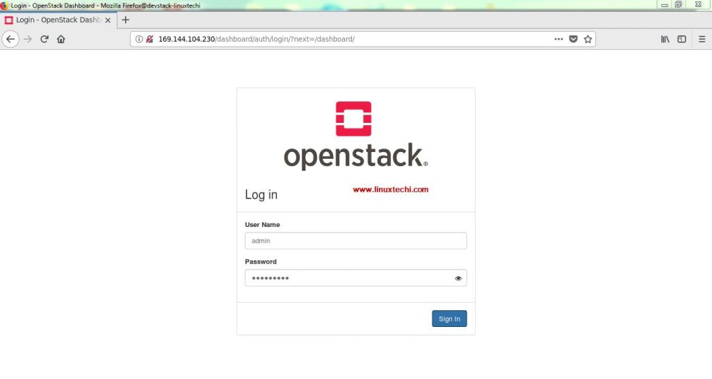
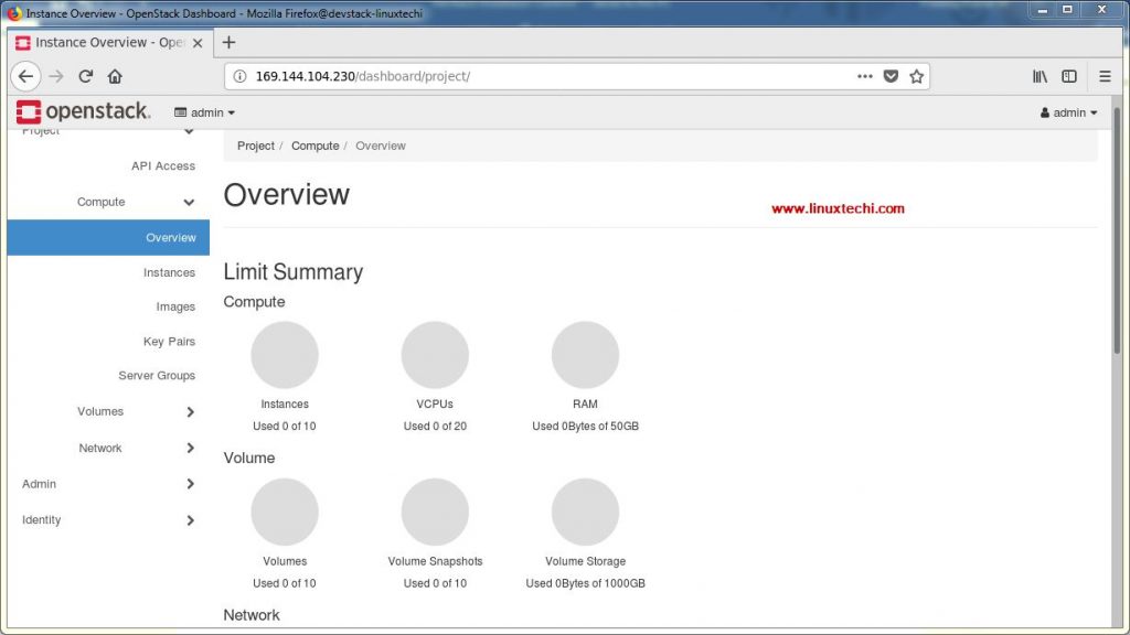
Now Try accessing the Horizon Dashboard, URL details and Credentials are already there in stack command output.

http://{Your-Server-IP-Address}/dashboard

Remove/ Uninstall OpenStack using devstack scripts

If are done with testing and demonstration and want to remove openstack from your system then run the followings scripts via Stack user,

[stack@devstack-linuxtechi ~]$ cd devstack
[stack@devstack-linuxtechi devstack]$ ./clean.sh
[stack@devstack-linuxtechi devstack]$ ./unstack.sh
[stack@devstack-linuxtechi devstack]$ rm -rf /opt/stack/
[stack@devstack-linuxtechi ~]$ sudo rm -rf devstack
[stack@devstack-linuxtechi ~]$ sudo rm -rf /usr/local/bin/

That’s all from this tutorial, if you like the steps, please do share your valuable feedback and comments.

Source

OOP doesn’t imply using function pointers.

The essence of OOP is polymorphism, which you can achieve in C through function pointers.

What about just having a plain structure and associate functions to it ? This is OO. In C, it forces you to adopt conventions like prefixing all your function names with the class name,…

I assume you’re refering to encapsulation, and I don’t see having to adopt a convention of prefixing your function with a object name (you’re not forced to) is a big deal unless you hunt and peck.

…and explicitely dereference all the member variables whenever you access them.

I assume you’re referring to having to pass in a pointer to structure and then using -> to dereference within a function. I don’t see how that’s a problem.

What about access rights ? There’s no way in C to forbid access to certain members of a structure. You have to document them in some way, by adding a comment next to the mmbers you consider private. And its not enforced by the compiler, thus errors can creep up.

Programmers should be using the public API. having public, protected, and private is no silver bullet.

Yes, programming using interface is useful, but there are lots of cases where objects with zero runtime overhead, but that implicitely do various housekeeping stuff, are very useful. Or even, classes that are there only to keep your code from getting full of long and messy functions, but amount to nothing at runtime.

Interfaces with virtual functions have a runtime cost, and these functions can’t be inlined. They’re not a silver bullet.

You don’t pay for what you don’t use in C also…unlike Java where you’re relying on the runtime to be smart about all methods being virtual.

And what about error management anyway ? You have to think of freeing resources everywhere, and C has no mechanism whatsoever to help you to do it. I don’t think it’s much better than an exception system, even if it has not so hard to avoid pitfalls.

Exceptions are useful, even though it has been pointed out that C++ exceptions have some major warts.

I understand your point, but I don’t think it’s really C++ fault. It’s more that since it allow to do these things more easily, it’s tempting to over-complicate stuff. I myself prefer straightforward code where I know what each classes actually do, and not have a vast amount of layers of abstraction if I don’t need them.

Yes, you can do everything in C that you do in C++, like object programming and stuff.

The purpose of C++ isn’t to let you do things that can’t be done in C, it’s to simplify your life. Indeed, it can complicate it instead, but not if used properly.

Pretty much agree on these points. Shallow hierarchies and favoring composition are the way to go.

I’ve written lots of C++ code in my lifetime (more than any other language). I think I somewhat grok proper OO. I’ve got Stroustrup’s 3rd edition I’ve got the GOF Design Patterns book, and think patterns are useful.

I guess my biggest problem with C++ is the syntax, the overcomplification of the language that seems to stem from it’s legacy of needing to be C-backward compatible, can’t stand C++ streams, and think much of the standard library API is bad.

Source

In this article, we will show you various useful ways of doing arithmetic’s in the Linux terminal. By the end of this article, you will learn basic different practical ways of doing mathematical calculations in the command line.

Let’s get started!

1. Using Bash Shell

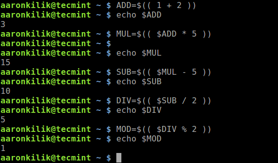
The first and easiest way do basic math on the Linux CLI is a using double parenthesis. Here are some examples where we use values stored in variables:

$ ADD=$(( 1 + 2 ))
$ echo $ADD
$ MUL=$(( $ADD * 5 ))
$ echo $MUL
$ SUB=$(( $MUL - 5 ))
$ echo $SUB
$ DIV=$(( $SUB / 2 ))
$ echo $DIV
$ MOD=$(( $DIV % 2 ))
$ echo $MOD

Arithmetic in Linux Bash Shell

2. Using expr Command

The expr command evaluates expressions and prints the value of provided expression to standard output. We will look at different ways of using expr for doing simple math, making comparison, incrementing the value of a variable and finding the length of a string.

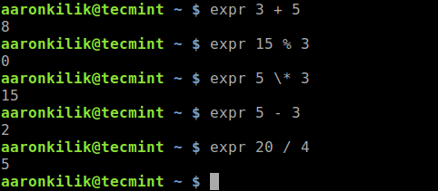
The following are some examples of doing simple calculations using the expr command. Note that many operators need to be escaped or quoted for shells, for instance the * operator (we will look at more under comparison of expressions).

$ expr 3 + 5
$ expr 15 % 3
$ expr 5 \* 3
$ expr 5 – 3
$ expr 20 / 4

Basic Arithmetic Using expr Command in Linux

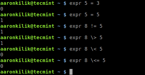
Next, we will cover how to make comparisons. When an expression evaluates to false, expr will print a value of 0, otherwise it prints 1.

Let’s look at some examples:

$ expr 5 = 3
$ expr 5 = 5
$ expr 8 != 5
$ expr 8 \> 5
$ expr 8 \< 5
$ expr 8 \<= 5

Comparing Arithmetic Expressions in Linux

You can also use the expr command to increment the value of a variable. Take a look at the following example (in the same way, you can also decrease the value of a variable).

$ NUM=$(( 1 + 2))
$ echo $NUM
$ NUM=$(expr $NUM + 2)
$ echo $NUM

Increment Value of a Variable

Let’s also look at how to find the length of a string using:

$ expr length "This is Tecmint.com"

Find Length of a String

For more information especially on the meaning of the above operators, see the expr man page:

$ man expr

3. Using bc Command

bc (Basic Calculator) is a command-line utility that provides all features you expect from a simple scientific or financial calculator. It is specifically useful for doing floating point math.

If bc command not installed, you can install it using:

$ sudo apt install bc   #Debian/Ubuntu
$ sudo yum install bc   #RHEL/CentOS
$ sudo dnf install bc   #Fedora 22+

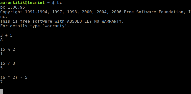
Once installed, you can run it in interactive mode or non-interactively by passing arguments to it – we will look at both case. To run it interactively, type the command bc on command prompt and start doing some math, as shown.

$ bc 

Start bc in Non-Interactive Mode

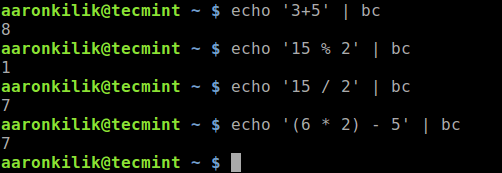
The following examples show how to use bc non-interactively on the command-line.

$ echo '3+5' | bc
$ echo '15 % 2' | bc
$ echo '15 / 2' | bc
$ echo '(6 * 2) - 5' | bc

Do Math Using bc in Linux

The -l flag is used to the default scale (digits after the decimal point) to 20, for example:

$ echo '12/5 | bc'
$ echo '12/5 | bc -l'

Do Math with Floating Numbers

4. Using Awk Command

Awk is one of the most prominent text-processing programs in GNU/Linux. It supports the addition, subtraction, multiplication, division, and modulus arithmetic operators. It is also useful for doing floating point math.

You can use it to do basic math as shown.

$ awk 'BEGIN { a = 6; b = 2; print "(a + b) = ", (a + b) }'
$ awk 'BEGIN { a = 6; b = 2; print "(a - b) = ", (a - b) }'
$ awk 'BEGIN { a = 6; b = 2; print "(a *  b) = ", (a * b) }'
$ awk 'BEGIN { a = 6; b = 2; print "(a / b) = ", (a / b) }'
$ awk 'BEGIN { a = 6; b = 2; print "(a % b) = ", (a % b) }'

Do Basic Math Using Awk Command

If you are new to Awk, we have a complete series of guides to get you started with learning it: Learn Awk Text Processing Tool.

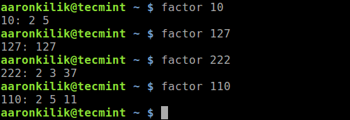
5. Using factor Command

The factor command is use to decompose an integer into prime factors. For example:

$ factor 10
$ factor 127
$ factor 222
$ factor 110  

Factor a Number in Linux

That’s all! In this article, we have explained various useful ways of doing arithmetic’s in the Linux terminal.

Source

Data compression is the process of storing data in a format that uses less space than the original representation would use. Compressing data can be very useful particularly in the field of communications as it enables devices to transmit or store data in fewer bits. Besides reducing transmission bandwidth, compression increases the amount of information that can be stored on a hard disk drive or other storage device.

There are two main types of compression. Lossy compression is a data encoding method which reduces a file by discarding certain information. When the file is uncompressed, not all of the original information will be recovered. Lossy compression is typically used to compress video, audio and images, as well as internet telephony. The fact that information is lost during compression will often be unnoticeable to most users. Lossy compression techniques are used in all DVDs, Blu-ray discs, and most multimedia available on the internet.

However, lossy compression is unsuitable where the original and the decompression data must be identical. In this situation, the user will need to use lossless compression. This type of compression is employed in compressing software applications, files, and text articles. Loseless compression is also popular in archiving music. This article focuses on lossless compression tools.

Popular lossless compression tools include gzip, bzip2, and xz. When compressing and decompressing files these tools use a single core. But these days, most people run machines with multi-core processors. You won’t see the speed advantage modern processors offer with the traditional tools. Step forward modern compression tools that use all the cores present on your system when compressing files, offering massive speed advantages.

Some of the tools covered in this article don’t provide significant acceleration when decompressing compressed files. The ones that do offer significant improvement, using multiple cores, when decompressing files are pbzip2, lbzip2, plzip, and lrzip.

Let’s check out the multi-core compression tools. See our time and size charts. And at the end of each page, there’s a table with links to a dedicated page for each of the multi-core tools setting out, in detail, their respective features.

Learn more about the features offered by the multi-core compression tool. We’ve compiled a dedicated page for each tool explaining, in detail, the features they offer.

With Default Compression

Default compression refers to running the compression tool without any compression flag being applied.

pigz compressed our 537MB tarball on our quad-core machine in the quickest time of all the tools, completing the test in a swift 4 seconds. To put the result into some context, we also ran the same test using gzip, which compressed the file in 14.7 seconds. pigz therefore fell a bit short of being 4x quicker.

You’ll notice lbzip2 and pbzip2 bars are colored red. This is because these tools use the best compression as their default.

pigz compressed the 537MB tarball down to 110MB. lrzip offers the best compression ratio for the tarball, squeezing it down to a frugal 64MB, although there isn’t much difference between lrzip, pxz, pixz, or plzip.

Again lbzip2 and pbzip2 bars are colored red. This is because these tools use the best compression as their default.

Methodology used for the tests

We took a 537MB tarball of a popular source package. The tarball was copied to RAM (/dev/shm), and the tests ran in RAM on a quad-core CPU without hyper-threading (Core i5-2500K), with no X server running, and under negligible load.

Each test was run three times with the latest version (at the time of writing) of each multi-core compression tool. The average results are recorded in the charts above. The tests show the relative difference between the multi-core compression tools. They are for indicative purposes only.

With Fastest Compression

Most of the tools provide a flag to set the level of compression on a scale from 1 to 9. pxz and plzip and pixz scale from 0 to 9. This test uses the lowest available compression option.

All of the multi-core tools made fairly light work of compressing the tarball with their fastest compression option.

If you need to compress large files on a machine with a low powered multi-core machine, the fastest compression might be suitable. pigz compressed the 537MB tarball to 134MB in a whisker under 1.7 seconds. Most of the other tools shaved the tarball to around 100MB, and lrzip compressed the file to a mere 90MB.

Methodology used for the tests

We took a 537MB tarball of a popular source package. The tarball was copied to RAM (/dev/shm), and the tests ran in RAM on a quad-core CPU without hyper-threading (Core i5-2500K), with no X server running, and under negligible load.

Each test was run three times with the latest version (at the time of writing) of each multi-core compression tool. The average results are recorded in the charts above. The tests show the relative difference between the multi-core compression tools. They are for indicative purposes only.

With Best Compression

The time taken to complete this test using the best compression option varies significantly within our group of tools. The fastest software is lbzip2 and pigz, both completing the task in under 9 seconds.

plzip is the slowest of the group taking nearly 100 seconds.

If space is paramount, pxz, plzip, pixz and lrzip offer impressive compression ratios. But pxz and pixz are quicker to complete.

Recent versions of pigz include the Zopfli engine which achieves higher compression than other zlib implementations but takes much longer to complete the compression. pigz uses Zopfli with the -11 flag.

Using Zopfli, pigz takes a whopping 14 minutes 25 seconds to complete the test. And while the compression ratio is better, the compressed file weights in at 104MB (as opposed to 109MB with the -9 flag). That’s still larger than the output from most of the multi-core tools with their fastest compression option.

pxz also has an extreme option which is triggered with the -e flag. Using the extreme option is designed to improve the compression ratio by using more CPU time. But compression ratio wasn’t improved in our tests. With the -9 flag, the tarball is 62MB. Yet, using the -e flag, the tarball was 65MB. We’ll need to run more tests to determine if this is just an anomaly.

Methodology used for the tests

We took a 537MB tarball of a popular source package. The tarball was copied to RAM (/dev/shm), and the tests ran in RAM on a quad-core CPU without hyper-threading (Core i5-2500K), with no X server running, and under negligible load.

Each test was run three times with the latest version (at the time of writing) of each multi-core compression tool. The average results are recorded in the charts above. The tests show the relative difference between the multi-core compression tools. They are for indicative purposes only.

Long Range Zip (Lrzip)

Lrzip uses an extended version of rzip, which does a first pass long distance redundancy reduction. It uniquely offers a good range of compression methods:

• LZMA (the default algorithm) – this is the Lempel–Ziv–Markov chain algorithm.
• ZPAQ – designed for user-level backups.
• LZO – Lempel–Ziv–Oberhume.
• gzip – based on the DEFLATE algorithm, which is a combination of LZ77 and Huffman coding.
• bzip2 – compression program that uses the Burrows–Wheeler algorithm.

When it comes to the size of the compressed tarball, zpaq offers the best compression.

Methodology used for the tests

We took a 537MB tarball of a popular source package. The tarball was copied to RAM (/dev/shm), and the tests ran in RAM on a quad-core CPU without hyper-threading (Core i5-2500K), with no X server running, and under negligible load.

Each test was run three times with the latest version (at the time of writing) of each multi-core compression tool. The average results are recorded in the charts above. The tests show the relative difference between the multi-core compression tools. They are for indicative purposes only.

Source

In this lesson on Python NumPy library, we will look at how this library allows us to manage powerful N-dimensional array objects with sophisticated functions present to manipulate and operate over these arrays. To make this lesson complete, we will cover the following sections:

• What is Python NumPy package?
• NumPy arrays
• Different operations which can be done over NumPy arrays
• Some more special functions

What is Python NumPy package?

Simply put, NumPy stands for ‘Numerical Python’ and that is what it aims to fulfil, to allow complex numerical operations performed on N-dimensional array objects very easily and in an intuitive manner. It is the core library used in scientific computing, with functions present to perform linear algebraic operations and statistical operations.

One of the most fundamental (and attractive) concepts to NumPy is its usage of N-dimensional array objects. We can take this array as just a collection of rows and column, just like an MS-Excel file. It is possible to convert a Python list into a NumPy array and operate functions over it.

NumPy Array representation

Just a note before starting, we use a virtual environment for this lesson which we made with the following command:

Once the virtual environment is active, we can install numpy library within the virtual env so that examples we create next can be executed:

We see something like this when we execute the above command:

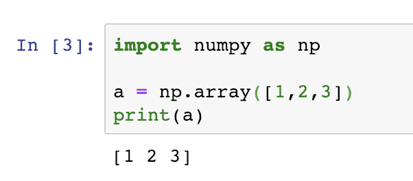
Let’s quickly test if the NumPy package has been installed correctly with the following short code snippet:

Once you run the above program, you should see the following output:

We can also have multi-dimensional arrays with NumPy:

This will produce an output like:

You can use Anaconda as well to run these examples which is easier and that is what we have used above. If you want to install it on your machine, look at the lesson which describes “How to Install Anaconda Python on Ubuntu 18.04 LTS” and share your feedback. Now, let us move forward to various types of operations that can be performed with with Python NumPy arrays.

Using NumPy arrays over Python lists

It is important to ask that when Python already has a sophisticated data structure to hold multiple items than why do we need NumPy arrays at all? The NumPy arrays are preferred over Python lists due to the following reasons:

• Convenient to use for mathematical and compute intensive operations due to presence of compatible NumPy functions
• They are much fast faster due to the way they store data internally
• Less memory

Let us prove that NumPy arrays occupy less memory. This can be done by writing a very simple Python program:

When we run the above program, we will get the following output:

This shows that the same size list is more than 3 times in size when compared to same size NumPy array.

Performing NumPy operations

In this section, let us quickly glance over the operations that can be performed on NumPy arrays.

Finding dimensions in array

As the NumPy array can be used in any dimensional space to hold data, we can find the dimension of an array with the following code snippet:

We will see the output as “2” as this is a 2-dimensional array.

Finding datatype of items in array

We can use NumPy array to hold any data type. Let’s now find out the data type of the data an array contains:

We used different type of elements in the above code snippet. Here is the output this script will show:

This happens as characters are interpreted as unicode characters and second one is obvious.

Reshape items of an array

If a NumPy array consists of 2 rows and 4 columns, it can be reshaped to contain 4 rows and 2 columns. Let’s write a simple code snippet for the same:

Once we run the above code snippet, we will get the following output with both arrays printed to the screen:

Note how NumPy took care of shifting and associating the elements to new rows.

Mathematical operations on items of an array

Performing mathematical operations on items of an array is very simple. We will start by writing a simple code snippet to find out maximum, minimum and addition of all items of the array. Here is the code snippet:

In the last 2 operations above, we also calculated the square root and standard deviation of each array items. The above snippet will provide the following output:

Converting Python lists to NumPy arrays

Even if you have been using Python lists in your existing programs and you don’t want to change all of that code but still want to make use of NumPy arrays in your new code, it is good to know that we can easily convert a Python list to a NumPy array. Here is an example:

Just to check, we can now print out the type of one of the variables:

And this will show:

We can now perform a mathematical operations over all the items at once. Let’s see how we can calculate the BMI of the people:

This will show the BMI of all the people calculated element-wise:

Isn’t that easy and handy? We can even filter data easily with a condition in place of an index inside square brackets:

This will give:

Create random sequences & repetitions with NumPy

With many features present in NumPy to create random data and arrange it in a required form, NumPy arrays are many times used in generating test dataset at many places, including debugging and testing purposes. For example, if you want to create an array from 0 to n, we can use the arange (note the single ‘r’) like the given snippet:

This will return the output as:

The same function can be used to provide a lower value so that the array starts from other numbers than 0:

This will return the output as:

The numbers need not be continuous, they can skip a fix step like:

This will return the output as:

We can also get the numbers in a decreasing order with a negative skip value:

This will return the output as:

It is possible to fund n numbers between x and y with equal space with linspace method, here is the code snippet for the same:

This will return the output as:

Please note that the output items are not equally spaced. NumPy does its best to do so but you need not rely on it as it does the rounding off.

Finally, let us look at how we can generate a set of random sequence with NumPy which is one of the most used function for testing purposes. We will pass a range of numbers to NumPy which will be used as an initial and final point for the random numbers:

The above snippet creates a 2 by 2 dimensional NumPy array which will contain random numbers between 0 and 10. Here is the sample output:

Please note as the numbers are random, the output can differ even between the 2 runs on the same machine.

Conclusion

In this lesson, we looked at various aspects of this computing library which we can use with Python to compute simple as well as complex mathematical problems which can arise in various use-cases The NumPy is one of the most important computation library when it comes to data engineering and calculating numerical dat, definitely a skill we need to have under our belt.

Source