 Welcome to the 2019 New Year’s edition catalog of hacker-friendly, open-spec SBCs that run Linux or Android. Here, we provide recently updated descriptions, specs, pricing, and links to details for all 122 SBCs.
Our New Year’s 2019 edition round-up of hacker-friendly, Linux or Android ready single board computers introduced six new entries since our June roundup for a total of 122 boards. This was even after we retired several older models like the 86Duino and PCDuino8 boards, which joined other boards that retired on their own, such as the Chip.
Newcomers range from amazingly affordable Rockchip RK3399 boards like the NanoPi Neo4 to the world’s first Intel Gemini Lake hacker board (Odroid-H2). There’s also an updated Raspberry Pi 3 Model A+ that gives you most of the features of the RPi 3 Model B+ in a smaller package.
The following summaries are listed in alpha order and are based on specs and lowest available pricing recorded in the last two weeks of Dec. 2018, with products either shipping or available for pre-order with expected ship date by the end of the month. Note: Summaries for SBCs that are new since our June reader survey edition SBC roundup are marked with a “NEW” tag. Another way to tour the catalog is by using one of the spreadsheet links above, which show comparative features and offer links to the blurbs below.Requirements for inclusion in the survey, which includes an under $200 price and significant open source support, may be found in our June catalog introduction. Results of the June reader survey may be found here.

- Mature, low-power Arm hacker board with GbE and 160 GPIOs
- Company/project — Olimex, OlinuXino, Mouser
- Product page
- Processor — Allwinner A20 (2x Cortex-A7 @ 1GHz); Mali-400 GPU
- Memory — 1GB DDR3 RAM; optional 4GB eMMC, 4GB NAND, or 8GB NAND flash
- Price — $51 (45 Euros); $63 (55 Euros) for 4GB version
Bulgaria-based Olimex’s OlinuXino project is one of the older hacker board projects around. Its aging A20-OlinuXino-Lime2 offers an Allwinner A20 with a Gigabit Ethernet (GbE, or 10/100/1000Mbps) port, microSD slot, HDMI port, LCD interface, and 3x USB ports. You also get battery support and 160 GPIOs. The 84 x 60mm SBC is available with Android 4.2.2 or Debian Jessie with Linux 3.4.1 mainline images.

- Optional industrial temp support and I/O expansion modules
- Company/project — Olimex, OlinuXino, Mouser
- LinuxGizmos report
- Product page
- Processor — Allwinner A20 (2x Cortex-A7 @ 1GHz); Mali-400 GPU
- Memory — 1GB DDR3 RAM; optional 4GB eMMC, 4GB NAND, and 8GB NAND
- Price — $63 (55 Euros); $74 (65 Euros) with 4GB eMMC
The A20-OlinuXino-Micro has all the I/O of the first-gen Lime models, and adds audio I/O, VGA, and an LCD interface with touch support. This larger, 142 x 83mm board offers expansion connectors with optional I/O modules. You get a choice of 4GB eMMC, 4GB NAND, and 8GB NAND versions, plus optional -45 to 85°C support on the microSD only and 4GB eMMC models.

- Smaller and less feature-rich than other Limes but with faster quad-core Allwinner A33
- Company/project — Olimex, OlinuXino, Mouser
- Product page
- Processor — Allwinner A33 (4x Cortex-A7 @ 1.2GHz); Mali-400 GPU
- Memory — 1GB DDR3 RAM; optional 4GB NAND
- Price — $41 (36 Euros) or $50 (44 Euros) for 4GB version
The 71 x 66mm A33-OlinuXino has a faster quad-core Allwinner A33 SoC compared to earlier OlinuXino boards, but it’s accompanied by a reduced feature set. The only real-world ports are a mini-USB OTG port, audio jacks, and a 5V jack. Two unassembled 40-pin connectors support GPIO, as well as 1280 x 800-pixel LCD and dual MIPI-CSI camera (5- and 8-megapixel) interfaces. Other features include a debug connector, a LiPo charger, and a step-up converter. You can download images for Android 4.4 and Armbian.

- First 64-bit OLinuXino
- Company/project — Olimex, OlinuXino, Mouser
- LinuxGizmos report
- Product page
- Processor — Allwinner A64 (4x Cortex-A53 @ 1.2GHz); Mali-400 MP2 GPU
- Memory — 1GB DDR3 RAM (2GB on 2G16G-IND ext. temp model); optional 4GB eMMC (16GB eMMC on 2G16G-IND)
- Price — $46 (40 Euros); $57 (50 Euros) for 4GB eMMC; $86 (75 Euros) for 2G16G-IND
Like Olimex’s open source (Teres-A64) laptop, the 90.0 x 62.5mm A64-OLinuXino runs Ubuntu/Linaro on a quad Cortex-A53 Allwinner A64. The A64-OLinuXino is available in three models: a 1G0G version with 1GB RAM and no flash, a 1G4GW with 1GB RAM and 4GB eMMC, and a 2G16G-IND with 2GB RAM, 16GB eMMC and -45 to 85°C support. The 4GB model, which is still the only one currently in stock, is also the only one with WiFi and Bluetooth. All three A64-OLinuXino models offer GbE, microSD, USB 2.0 host, micro-USB OTG, HDMI, and MIPI-DSI connections. Interfaces including LCD and MIPI-CSI are accessible via the 40-pin GPIO connector. Other extras include an RTC and a LiPo battery connector with step-up and charging support.

- Reboot of the original Linux-driven Arduino board
- Company/project — Arduino
- LinuxGizmos report
- Product page
- Processor — Qualcomm Atheros AR9331 (1x MIPS 24kc @ 400MHz); Atmel ATmega32u4 MCU @ 16MHz
- Memory — 64MB RAM; 16MB flash; 32KB flash for MCU
- Price — $59
 Just when we thought Arduino was done with its Linux experimentation, the company returned with a reboot of its original, MIPS-based Arduino Yun. Like the original it combines a WiFi-enabled, 400MHz AR9331 SoC running OpenWrt Linux with an ATmega32U MCU that runs Arduino code. The board is once again equipped with a microSD slot and USB host, micro-USB, and 10/100 Ethernet ports. Improvements have been made to the LAN and USB components, and you now get SSL support for improved security.

- Raspberry Pi sized variant of BPI-M2 Ultra with native SATA and camera support
- Company/project — SinoVoip
- LinuxGizmos report
- Product page
- Processor — Allwinner V40 (4x Cortex-A7); Mali-400 MP2 GPU
- Memory — 1GB DDR3 RAM
- Price — $36
The Banana Pi BPI-M2 Berry is one of several new Banana Pi models to ship over the last year. There have been no new has shown up since our June roundup, although Sinovoip posted specs for two boards this summer that have yet to ship: the Banana Pi BPI-P2 Zero and Banana Pi BPI-R64. The BPI-M2 Berry is based on the earlier BPI-Ultra design, and similarly offers native SATA support (see below). The Berry is smaller, with a Raspberry Pi-like 85 x 56mm footprint, and has a different quad -A7 Allwinner SoC: the camera enabled Allwinner V40 in place of the almost identical R40. The Berry lacks the Ultra’s eMMC storage, and it offers 1GB DDR3 instead of 2GB. In place of a 5V jack, you draw power via micro-USB OTG, and you won’t find the Ultra’s battery support, IR receiver, or debug UART. On the other hand, the Berry adds a fourth USB 2.0 host port and a MIPI-CSI camera connector. Other features include microSD, WiFi, Bluetooth, GbE, HDMI, MIPI-DSI, and audio connections, as well as an RPi-compatible 40-pin expansion.

- Tiny quad-core board features MIPI-DSI and -CSI takes
- Company/project — SinoVoip
- LinuxGizmos report
- Product page
- Processor — Allwinner A33 (4x Cortex-A7); Mali-400 MP2 GPU
- Memory — 512MB DDR3 RAM; 8GB eMMC (optional 16GB, 32GB, or 64GB)
- Price — $28
Available for $28 on Alibaba, the Banana Pi BPI-M2 Magic (BPI-M2M), has a 51 x 51mm footprint that puts it in the same league as the tiny NanoPi Neo boards. The BPI-M2 Magic runs Debian, Ubuntu, Android, or a Raspberry Pi image on an Allwinner A33, and offers WiFi, BT, and a microSD slot to augment its 8GB and up eMMC. You also get USB and micro-USB OTG ports and a 40-pin RPi header. Media interfaces include MIPI-DSI and -CSI, an audio jack, and an onboard mic.

- BPI-M2 upgrade adds native SATA and 2GB of RAM
- Company/project — SinoVoip
- LinuxGizmos report
- Product page
- Processor — Allwinner R40 (4x Cortex-A7); Mali-400 MP2 GPU
- Memory — 2GB DDR3 RAM; 8GB to 64GB eMMC
- Price — $56
The Banana Pi M2 Ultra (BPI-M2U) can be found for a low of $56 on Amazon. It upgrades the similarly 92 x 60mm BPI-M2 and offers a faster Allwinner R40, which enables a native SATA connector. You get a generous 2GB of RAM, which is unusual for a Cortex-A7 SoC. The M2 Ultra is further equipped with GbE, WiFi, Bluetooth, 3x USB host, and single HDMI and micro-USB OTG ports. A 40-pin connector supports Raspberry Pi add-ons, and you get MIPI-DSI, an audio jack, and a mic interface.

- Raspberry Pi Zero W pseudo clone
- Company/project — SinoVoip
- LinuxGizmos report
- Product page
- Processor — Allwinner H2+ (4x Cortex-A7 @ 1.2GHz); Mali-400 MP2 GPU
- Memory — 512MB DDR3 RAM
- Price — $22.90
Selling for $22.90 on AliExpress, the 60 x 30mm Banana Pi BPI-M2 Zero mimics the Raspberry Pi Zero W, but has a faster Allwinner H2+, which is like an Allwinner H3, but with HD instead of 4K support. The feature set is almost identical, with WiFi, BT, MIPI-CSI, 40-pin RPi expansion, and mini-HDMI and power-only micro-USB OTG ports. In August, Sinovoip posted specs for a still unavailable spinoff of the M2 Zero called the BPI-P2 Zero that adds 8GB eMMC and 10/100 Ethernet with PoE.

- Feature-rich, 32-bit octa-core SBC with SATA and extensive OS support
- Company/project — SinoVoip
- Product page
- Processor — Allwinner A83T (8x Cortex-A7 @ 1.8GHz); PowerVR SGX544MP1 GPU
- Memory — 2GB LPDDR3 RAM; 8GB to 64GB eMMC
- Price — $99
The Banana Pi M3 (BPI-M3) sekks for $99 on AliExpress, which is up by $20 since June. This high-end board features the octa-core Allwinner A83T SoC, backed up with 2GB RAM and 8GB eMMC. The M3 has about the same size (92 x 60mm), layout, and features of the M2 Ultra, and similarly integrates a RPi-ready 40-pin link. Like the M2 Ultra, the M3 supplies GbE, WiFi, SATA, 3x USB, and multiple display and camera options. Software support is more extensive than with some other Banana Pi boards, although all have improved. Options include Android 5.1, Debian 8, Ubuntu 16.04 Mate, Raspbian Jesse Mate, and much more.

- First 64-bit Banana Pi offers 2GB RAM and 4K video
- Company/project — SinoVoip
- LinuxGizmos report
- Product page
- Processor — Allwinner A64 (4x Cortex-A53 @ 1.2GHz); Mali-400 MP2 GPU
- Memory — 2GB DDR3 RAM; 8GB to 64GB eMMC
- Price — $68
SinoVoip’s only 64-bit Banana Pi sells for $68 at AliExpress, which is pricier than the similarly Allwinner A64-equipped Pine A64. On the other hand, the Banana Pi BPI-M64 is loaded with 2GB RAM and 8GB eMMC, as well as numerous peripherals. You get 4K-ready HDMI, MIPI-DSI, and MIPI-CSI, as well as onboard wireless and GbE connections. The 92 x 60mm board is further equipped with 3x USB host ports, a micro-USB OTG port, and an RPi 40-pin connector.

- Router board offers 4x GbE ports, up to 2x SATA, and mini-PCIe 2.0
- Company/project — SinoVoip
- LinuxGizmos report
- Product page
- Processor – MediaTek MT7623N (4x Cortex-A7 @ 1.3GHz); Mali-450 MP4 GPU
- Memory — 2GB DDR3 RAM; 8GB eMMC
- Price — $89.50
The BPI-R2 follow-on to the popular BPI-R1 router board was announced a year ago and is now shipping for $104 at Amazon and $89.50 at AliExpress. Like the R1, the R2 offers 4x GbE ports and a WAN port, as well as HDMI 1.4 out and MIPI-DSI outputs. The R2 has a faster, more network-capable quad -A7 MediaTek MT7623N SoC plus more RAM and storage and the option for a second SATA III interface. It also adds Bluetooth, mini-PCIe, 40-pin GPIO, and improved USB support: 2x USB 3.0 host and a micro-USB 2.0 OTG. The upcoming Banana Pi BPI-R64 will not be a clear upgrade. It offers a more network savvy, Cortex-A53 based MT7622 SoC, but there’s no GPU and only two CPU cores. The BPI-R64 will have no video outputs and is limited to only 1GB of RAM and single USB and SATA connections. The BPI-R64 will have the same 148 × 100.5mm dimensions as the R1 and R2, and most of the same features of the R2.

- Under $100 router board features dual SATA III, dual GbE, and triple M.2
- Company/project — SinoVoip
- LinuxGizmos report
- Product page
- Processor — Realtek RTD1296 (4x Cortex-A53 @ up to 1.5GHz); Mali-T820 MP3 GPU
- Memory — 2GB DDR4 RAM; 8GB to 64GB eMMC
- Price — $93
The Banana Pi BPI-W2 ripened to maturity in April on AliExpress, where it sells for $93. This 148 x 100.5mm router and NAS board is a spinoff to the R1 and R2 boards listed above. It provides dual SATA III, dual GbE, and a WAN port. You also get 4x USB, including Type-C and 3.0 host ports. For expansion there are 3x M.2 slots with PCIe support and a SIM slot, as well as a 40-pin RPi-style connector. Unlike most networking-focused boards, the BPI-W2 can also bring it when it comes to multimedia: You get HDMI in and out, a mini-DisplayPort, and an audio jack. The BPI-W2 runs Android 6.0, CentOS, Debian 9, Raspbian, Ubuntu 15.04, or OpenWrt on Realtek’s RTD1296, a NAS-oriented variant of the RTD1295 with a powerhouse Mali-T820 MP3 GPU. For other open-spec NAS alternatives you can keep an eye on Kobol’s
Helios4 with a Marvell Armada 388 SoC and 4x SATA slots. The Helios4 relaunched in July, but it is already sold out, and the only model that appears as if it might return to pre-order is a
full kit system with enclosure and fan selling for $194.44.

- Open source legend focuses on industrial I/O — and community
- Company/project — BeagleBoard.org
- LinuxGizmos report
- Product page
- Processor — TI Sitara AM3358 (1x Cortex-A8 @ 1GHz) with PRU MCU chips; PowerVR SGX530 GPU
- Memory — 512MB RAM; 4GB eMMC
- Price — $55
The industrial-oriented, Debian-ready BeagleBone Black Rev C stands out with its numerous expansion interfaces and programmable “PRU” MCUs, as well as its deeply rooted BeagleBoard.org community. This legendary hacker board is currently available for $55 at Arrow or Mouser while Element14 nips the price down to $53.64. The BB Black has been followed by more feature rich and/or lower cost clones that have been created or approved by BeagleBoard.org. Yet, the original still came in 6th out of 116 SBCs in our June reader survey. Farther below, check out our reports on two BeagleBone Green models from Seeed, as well as BeagleBoard.org’s own BeagleBone Black Wireless, BeagleBone Blue, and new PocketBeagle. Element14’s BeagleBone Black Industrial 4G, which is identical to the BB Black except for its conformal coating and -20 to 85°C support, is usually out of stock, but we found it selling for $92.14 at AliExpress.
| BeagleBone Black Wireless |

- SiP-based BeagleBone Black follow-on with wireless and HDMI, but no Ethernet
- Company/project — BeagleBoard.org; Octavo Systems
- LinuxGizmos report
- Product page
- Processor — Octavo Systems OSD3358 SiP with TI Sitara AM3358 (1x Cortex-A8 @ 1GHz) with PRU MCUs; PowerVR SGX530 GPU
- Memory — 512MB RAM; 4GB eMMC
- Price — $68.75
BeagleBoard.org’s alternative to Seeed’s BeagleBone Green Wireless similarly adds 2.4GHz 802.11a/b/g/n and Bluetooth 4.1 BLE to the BeagleBone Black design. Unlike Seeed’s two BB Green models, the BeagleBone Black Wireless retains the BB Black’s micro-HDMI port, but removes the Ethernet port. It is otherwise identical to the BB Black with one big exception: It incorporates the OSD3358 SiP (system-in-package) module from Octavo Systems, which built the SBC as well. (SiPs simplify board development and make it easier to create custom variations.) Also see Octavo’s own OSD3358-SM-RED, a more advanced BeagleBone compatible dev board with the same SiP package.

- Robotics and STEM focused BeagleBone with servos, sensors, and wide-range power
- Company/project — BeagleBoard.org
- LinuxGizmos report
- Product page
- Processor — Octavo Systems OSD3358 SiP with TI Sitara AM3358 (1x Cortex-A8 @ 1GHz) with PRU MCU chips and PowerVR SGX530 GPU
- Memory — 512MB RAM; 4GB eMMC
- Price — $80
This robotics-oriented, education-focused BeagleBoard.org collaboration with the UCSD Coordinated Robotics Lab is a BeagleBone clone that adds motion control and battery friendly power. It sells for a low of $80 at Arrow and Element14. Like the BeagleBone Black Wireless, the BeagleBone Blue integrates a TI WiLink 8 with WiFi and Bluetooth 4.1 LE, as well as an Octavo Systems OSD3358 SiP module that encapsulates the Sitara AM3358 SoC, RAM, and flash along with a PMIC and other features. There’s no Ethernet port or display interfaces, but you get micro-USB 2.0 host and client ports, 8x servo outputs, 4x DC motor outputs, and 4x quad encoder inputs. Other features include an IMU, barometer, JTAG, GPS, and DSM2 radio. You also get a 9-18V DC input, a LiPo battery connector, extra user buttons and LEDs, plus the usual extensive list of BB Black interfaces. Distro support includes the usual real-time enhanced Debian stack, as well as Ubuntu Core, ROS, and ArduPilot.

- IoT-focused BeagleBone clone with Grove sensor support
- Company/project — Seeed; BeagleBoard.org
- LinuxGizmos report
- Product page
- Processor — TI Sitara AM3358 (1x Cortex-A8 @ 1GHz) with PRU MCU chips; PowerVR SGX530 GPU
- Memory — 512MB RAM; 4GB eMMC
- Price — $44
Seeed’s BeagleBoard.org-sanctioned, IoT-focused re-spin of the BeagleBone Black lacks the BB Black’s micro-HDMI port and 5V barrel jack, but it costs less, and adds expansion connectors for Seeed’s Grove sensors. It also replaces the mini-USB port with a micro-USB. In addition to drawing on the support of BeagleBoard.org, you can find a Grove-oriented BB Green developer site at Seeed.
| BeagleBone Green Wireless |

- Wireless version of BeagleBone Green with 4x USB host ports
- Company/project — SeeedStudio; BeagleBoard.org
- LinuxGizmos report
- Product page
- Processor — TI Sitara AM3358 (1x Cortex-A8 @ 1GHz) with PRU MCU chips; PowerVR SGX530 GPU
- Memory — 512MB RAM; 4GB eMMC
- Price — $52.90
The BeagleBone Green Wireless has the same base feature set as the BB Green, with identical additions and subtractions from the BB Black, including the addition of a Grove interface. The Wireless model adds WiFi and Bluetooth, as well as three more USB host ports for a total of four, making it the USB leader among all the BB Black clones. A TI WiLink8 module is now standard, boosting wireless capabilities to Bluetooth 4.1 LE and 2.4GHz 802.11a/b/g/n with 2×2 MIMO.

- Affordable 96Boards CE board with 2GB RAM
- Company/project — uCRobotics
- LinuxGizmos report
- Product page
- Processor — Actions Semiconductor Actions S900 (4x Cortex-A53 @ 1.8GHz); PowerVR G6230 GPU
- Memory — 2GB LPDDR3 RAM; 8GB eMMC
- Price — $89
uCRobotics’ Bubblegum-96 is a 96Boards CE form-factor board with 2GB RAM. Aside from the 96Boards 40- and 60-pin expansion connectors, the affordably priced Bubblegum-96 supplies an HDMI port, a microSD slot, a micro-USB port, and dual USB host ports, one of which is USB 3.0. WiFi and Bluetooth are also available.
| C-SKY Linux Development Board |

- Low-cost IoT board showcases SoC with new C-SKY ISA
- Company/project — Hangzhou C-SKY
- LinuxGizmos report
- Product page
- Processor — Nationalchip GX6605S CK610M (1x C-SKY @ 574MHz)
- Memory — 64MB DDR2 RAM
- Price — $5.60 and up
It doesn’t cost much to try out the new C-SKY ISA launched in China by Hangzhou C-SKY. The C-SKY Linux Development Board, which debuts the Nationalchip GX6605S SoC, sells for less than $6 on Taobao and $18.33 on AliExpress. The mainline Linux Kernel now supports the new ISA, and the board is supported with a Linux 4.16 based stack with Buildroot and uClibc-NG. Schematics are also available. The C-SKY dev board is a bit smaller than a Raspberry Pi and offers an HD-ready HDMI port and dual USB 2.0 ports. One of the two micro-USB ports supports JTAG debugging and the other offers 5V/1A power with UART console. A 5-pin header offers power and 3x GPIO, and you get a reset button and several user buttons and LEDs.

- Security-enhanced 96Boards CE board with Cyclone V SE FPGA SoC and dual-stream video
- Company/project — Novtech, Arrow, RocketBoards.org
- LinuxGizmos report
- Product page
- Processor — Intel Cyclone V SE SoC (2x Cortex-A9); Cyclone V FPGA with 110K LEs
- Memory — 512MB or 1GB DDR3 RAM
- Price — $145
Novtech’s 96Boards CE compatible Chameleon96 SBC is available for $145 at Arrow, up from $129 in June. The very first FPGA-based 96Boards entry runs Debian on a Cyclone V SE ARM/FPGA SoC. The Chameleon96 is notable for providing SecureRF’s quantum-resistant security and FPGA-driven video. The Intel Video Suite for FPGA technology can drive 60fps 1080p streams via the HDMI port, and can encode similar video via a two-lane MIPI-CSI camera interface. Other features include a microSD slot, a micro-USB OTG port, 2x USB 2.0 host ports, an audio interface, a USB Blaster, and a UART. Like most 96Boards SBCs, this 12V SBC offers WiFi and Bluetooth, but lacks Ethernet. It offers the usual 96Boards low- and high-speed I/O connectors.

- Kit features miniature ARM9 IoT board and lets you add LittleBits modules
- Company/project — LittleBits Electronics
- LinuxGizmos report
- Product page
- Processor — NXP i.MX233 (1x ARM9 @ 454MHz)
- Memory — 64MB RAM; 4GB microSD card
- Price — $65
The lone Linux board in the Arduino-oriented LittleBits maker platform is one of the smallest SBCs around at 15 x 10mm. The boardlet integrates WiFi, a power-only micro-USB port, and dual “BitSnap” connectors for adding standard LittleBits modules. The CloudBit is sold out at LittleBits, but a Cloudbit Starter Kit that offers the CloudBit with five prototyping modules is available at Walmart for $65. The Arch Linux based platform supports IFTTT scripting and connects to a Node.js-oriented cloud platform designed for monitoring IoT gizmos. This is the only board in the roundup with a processor based on the ancient, low power ARM9 architecture.

- A turbo-charged version of the CubieAIO-A20 that moves to a quad -A53 Actions S700
- Company/project — CubieBoard.org, CubieTech Limited
- LinuxGizmos report
- Product page
- Processor — CubieTech Actions S700 (4x Cortex-A53); Mali-450 MP4 GPU
- Memory — 2GB LPDDR3 RAM; 8GB eMMC
- Price — $139
In July 2017, CubieTech became an official distributor of the application processor unit of Actions Technology, and later announced several Actions-based open source SBCs. The sandwich-style CubieAIO-S700 features the quad-A53 Actions S700 via CubieTech’s Einstein-S700 module, which integrates an Ampak AP6212 chip with WiFi-ac and BT 4.0. Aside from the different Einstein processor module, the board is a very close match in features and layout with the apparently discontinued, Allwinner A20 based CubieAIO-A20. The 170 x 106mm SBC has a high, 20mm profile due to its 6x, double-stacked USB 2.0 host ports. The HDMI port tops out at HD resolution, but you get a GbE port, SPDIF audio, dual coastline serial ports, a SIM slot, and dual mini-PCIe slots, one of which has non-native mSATA. The CubieAIO-S700 also has a 54-pin expansion header, RTC, IR, and more. The full CubieAIO-S700 kit starts at $139 at AliExpress. CubieTech has also posted details for a CubieAIO-S500 SBC which is almost identical to the CubieAIO-S700 but has an Einstein S500 module with a quad -A9 Actions S500 SoC. The board has yet to reach market.

- Feature-rich, octa-core -A15 board with multiple storage options
- Company/project — CubieBoard.org, CubieTech Limited
- LinuxGizmos report
- Product page
- Processor — Allwinner A80 (4x Cortex-A15 @ up to 2GHz, 4x Cortex-A7 @ up to 1.3GHz); PowerVR G6230 GPU
- Memory — 2GB DDR3 RAM; 8GB eMMC, expandable to 64GB
- Price — $129.90
The CubieBoard4 is equipped with an octa-core Allwinner A80 SoC with a 64-core PowerVR G6230 GPU. The 111 x 111mm SBC offers WiFi, Bluetooth, and GbE, as well as VGA, HDMI, USB 3.0, and 4x USB 2.0 ports. There’s also a 54-pin expansion connector. The SBC provides optional configurations including dual microSD slots or a mix of microSD and onboard flash. There are plenty of cases and other add-ons, as well as images for Debian, Ubuntu, and Android, with mainline Linux support. The boards costs $129.90 at Amazon.
| CubieBoard5 (CubieTruck-Plus) |

- Octa-core -A7 board with SATA and dual display support
- Company/project — CubieBoard.org, CubieTech Limited
- Product page
- Processor — Allwinner H8 (8x Cortex-A7 @ up to 2GHz); PowerVR SGX544 GPU @ up to 700MHz
- Memory — 2GB DDR3 RAM
- Price — $105
The CubieBoard5, which sells for $105 at Amazon, showcases an Allwinner H8 with eight Cortex-A7 cores. The SBC provides microSD and SATA storage, with an optional RAID add-on board. For connectivity, you get WiFi, Bluetooth 4.0, and a GbE port. Dual display support is available via the HDMI and DisplayPorts. The board is further equipped with a pair of USB host ports, an IR sensor, S/PDIF audio, and an optional lithium battery.
| CubieBoard6 / CubieBoard7 |

- Monolithic cousins to the sandwich style CubieAIO boards with faster SATA and USB 3.0
- Company/project — CubieBoard.org, CubieTech Limited
- LinuxGizmos report
- Product page
- Processor — CubieBoard6: CubieTech Actions S500 (4x Cortex-A9 @ 1.2GHz, PowerVR SGX544 GPU); CubieBoard7: CubieTech Actions S700 (4x Cortex-A53, Mali-450 MP4 GPU)
- Memory — 2GB LPDDR3 RAM; 8GB eMMC
- Price — $89 (CubieBoard6); $99 (CubieBoard7)
The new CubieBoard6 and CubieBoard7 SBCs, which are identical except for their processors, are the monolithic cousins to the sandwich-style CubieAIO-S500 and CubieAIO-S700, respectively. These updates to the four-year old CubieBoard2 have smaller 100 x 60mm footprints compared to the CubieAIO boards, as well as a lesser feature set. The key advantage in addition to their lower prices is that their non-native SATA ports piggyback on a faster USB 3.0 connection to offer an approximation of SATA III. The boards provide 10/100 Ethernet, 802.11n, and BT 4.0, as well as 2x USB 2.0 host ports and a mini-USB port. Other features include HD-ready HDMI, audio jacks, RTC, IR, a UART header, and dual 48-pin expansion headers. Like the CubieAIO boards, they are supported with Actions-optimized Android 5.1.1 and Debian builds. The CubieBoard6 sells for $89 and the CubieBoard7 for $99, both at AliExpress. This year, CubieTech posted a product page for a quad -A53 Actions S900 based CubieBoard9 replacement for the CubieBoard4, but it has yet to reach market.
| DE0-Nano-SoC Development Kit |

- Dev board features Cyclone V SE FPGA SoC and Arduino shield support
- Company/project — Terasic; RocketBoards.org
- Product page
- Processor — Intel Cyclone V SE (Cyclone V FPGA + 2x Cortex-A9 @ 952MHz)
- Memory — 1GB DDR3 RAM
- Price — $99
The DE0-Nano-SoC Development Kit looks like a commercial development board, but it offers open specifications and is supported on the RocketBoards.org community site. The DE0-Nano-SoC uses the lower-end SE variety of Intel’s Cyclone V SoC, which is roughly equivalent to a Xilinx Zynq-7020. The SoC similarly combines FPGA circuitry with dual Cortex-A9 cores running Angstrom v2014.12 Yocto 1.7 with a Linux 4.0 kernel. The board has GbE, USB OTG, and micro-USB ports, as well as a microSD slot with a 4GB data card. There’s also an accelerometer, an Arm-linked expansion header, and a variety of FPGA-linked interfaces, including a 40-pin header and an Arduino shield connector. (There’s also an identical “Atlas-SoC” variant that’s packaged for software rather than hardware developers.)

- Company/project — Arrow; Qualcomm
- Venerable 96Boards CE board returns to full production
- LinuxGizmos coverage
- Product page
- Processor — Snapdragon 410 (4x Cortex-A53 @ 1.2GHz); Adreno 306 GPU
- Memory — 1GB LPDDR3 RAM; 8GB eMMC
- Price — $75
Last June we prematurely pulled Arrow’s Qualcomm-backed DragonBoard 410c from our catalog in the belief the board was permanently out of stock. However, Arrow has ramped up production for this Qualcomm-backed SBC, which along with the now defunct HiKey, was not only the first 96Boards Consumer Edition (CE) SBC, but the first 64-bit ARM hacker SBC. At 85 x 54mm, this Snapdragon 410 driven SBC is about the same size as the Raspberry Pi. There’s no Ethernet port, but you get WiFi, Bluetooth, GPS, HDMI, microSD, 3x USB ports, and the 96Boards 40-pin low-speed and 60-pin high-speed connectors. The SBC supports Android 5.1, Debian 8.0, and Windows 10 IoT Core.

- 96Boards CE Extended board with high-end, AI-ready Snapdragon 820E
- Company/project — Arrow, 96Boards
- LinuxGizmos report
- Product page
- Processor — Qualcomm Snapdragon 820E (2x Kyro cores @ 2.35GHz, 2x @ 1.6GHz); Adreno 530 GPU, etc.
- Memory — 3GB LPDDR4-1866 RAM; 32GB UFS 2.0
- Price — $199
The DragonBoard 820c was launched earlier this year, but Arrow does not currently have a shopping page. We’ll include it here in the belief that a page will appear soon. Like the DragonBoard 410c, this is a 96Boards CE board, but it uses the larger Extended (100 x 85mm) variant. In addition to the CE standard 40- and 60-pin connectors, the Extended format supplies a second 60-pin high-speed connector with 4L-MIPI DSI, SSC serial, and TSIF, and provides a separate analog audio header. The board is based on the eInfochips SD 600eval SBC, which was equipped with a Snapdragon 600, and which Arrow had floated as a prototype called the DragonBoard 600c. The DragonBoard 820c was introduced as part of Linaro’s multi-board 96Boards.ai initiative. In this case, the AI is enabled via the Snapdragon 820E’s Spectra ISP, which supports Qualcomm’s Linux-driven Snapdragon Neural Processing Engine SDK. The DragonBoard 820c is equipped with 3GB LPDDR4-1866 RAM, 32GB UFS 2.0 UFS storage, HDMI 2.0, 2x USB 3.0, and a micro-USB OTG port. In addition to a GbE port, you get WiFi-ac, BT 4.2, GPS, an IMU, a magnetometer, and a wide-range power supply. Meanwhile, Geniatech has launched its own Snapdragon 820E based 96Boards SBC called the Developer Board 8, which is over our $200 limit.

- Sandwich-style board with new Rockchip PX3-SE SoC and -20 to 80℃ support
- Company/project – Firefly
- LinuxGizmos report
- Product page
- Processor — Rockchip PX3-SE (4x Cortex-A7 @ 1.3GHz); Mali-400 MP2 GPU
- Memory — 1GB RAM; 8GB eMMC
- Price — $60
The Firefly-PX3-SE is an extended temperature alternative to the Firefly-RK3128 with a similar quad -A7 SoC called the PX3-SE. Like the Firefly-RK3128, this is a sandwich-style board, with the SoC and RAM in this case implemented via a Core-PX3-SEJ module. Despite the lack of 4K support, there are a numerous media interfaces, including HDMI, CVBS, MIPI-DSI or LVDS, and DVP camera. For audio, you get analog, SPDIF, and I2S audio plus an onboard mic and a “phone” I/O port. The Firefly-PX3-SE board is further equipped with a GbE port, WiFi/BT, 4x USB 2.0, micro-USB OTG, 84-pin expansion header, RTC, debug, and IR. Android 5.1 and Ubuntu 15.04 are available. Although billed as an open source board, we have yet to see hardware documents posted on the download page.

- Feature-rich, sandwich-style board with aging Rockchip SoC gets steep discount
- Company/project — Firefly
- Product page
- Processor — Rockchip RK3128 (4x Cortex-A7 @ 1.3GHz); Mali-400 MP2 GPU
- Memory — 1GB RAM; 8GB NAND flash
- Price — $60
This low-end Firefly board is available at a $60 promotional price. The Firefly-RK3128 dual boots Android 5.1 and Ubuntu 15.04 on a quad-core -A7 Rockchip that is clocked slower than the RK3288 and offers half the RAM and flash of the Firefly-RK3288. The sandwich-style, COM/baseboard device includes GbE, WiFi, BT, HDMI, MIPI-DSI, MIPI-CSI, SPDIF, analog audio, LVDS, IR, and CVBS. The 117 x 85mm boardset is further equipped with 4x USB host ports, a micro-USB OTG port, and dual 42-pin expansion connectors. Firefly just introduced a similar, but extended temp SBC called the Firefly-PX3-SE (see above).

- Quad -A17 board with onboard wireless and 4K-ready HDMI 2.0
- Company/project — Firefly
- Product page
- Processor — Rockchip RK3288 (4x Cortex-A17 @ 1.8GHz); Mali-T760 GPU
- Memory — 2GB or 4GB DDR3 RAM; 16GB or 32GB eMMC
- Price — $119 (2GB/16GB); $189 (4GB/32GB)
Starting at $119, this 118 x 85mm SBC dual boots Ubuntu 14.04 and Android 4.4 with mainline Linux 4.4 support on a 1.8GHz, quad -A17 RK3288 with Mali-T760 GPU. The Firefly-RK3288 has an HDMI 2.0 port that can output at up to 4Kx2K @ 60Hz. The board offers dual-band 802.11ac, Bluetooth 4.0, a GbE port, and 3x USB ports, and is further equipped with VGA, LVDS, eDP, MIPI-DSI, MIPI-CSI, S/PDIF, serial debug, and IR connections. More I/O is available via dual 42-pin connectors. A “Fireasy” WiFi remote, as well as touchscreens, fans, and cameras, are optional.

- Sandwich-style version of Firefly-RK3288 adds SATA, an HDMI input, and more USB and GPIO
- Company/project — Firefly
- LinuxGizmos report
- Product page
- Processor — Rockchip RK3288 (4x Cortex-A17 @ 1.8GHz); Mali-T760 GPU
- Memory — 2GB DDR3 RAM; 16GB eMMC
- Price — $159
The Firefly-RK3288 Reload has the same SoC and OS support as the Firefly-RK3288 but is recast as a sandwich-style COM/baseboard product. The 178 x 117mm baseboard connects to the 82 x 60mm COM via a 314-pin MXM connector. The Reload provides all the features of the Firefly-RK3288, and adds a second HDMI output, a new HDMI input, and a second DVP interface for a 5MP camera in addition to the 13MP-ready DVP. The Reload also adds a SATA port, a third USB host, and a micro-USB OTG, and boosts the expansion pins to 184. The Reload’s COM is separately available as a $105 Firefly-RK3288 Reload CoreBoard, which is also available in a 189 x 107mm, sandwich-style “All-in-One” development platform called the AIO-3288J. The AIO-3288J lacks the Reload’s SATA port, and has two HDMI ports instead of three, yet it offers more onboard interfaces. It also sells for a lower $139 price, including the CoreBoard.

- Powerhouse RK3399-based hacker board with M.2, mini-PCIe, and dual 4K display ports
- Company/project — Firefly
- LinuxGizmos report
- Product page
- Processor — Rockchip RK3399 (2x Cortex-A72 @ up to 2.0GHz, 4x Cortex-A53 at up to 1.42GHz); Mali-T860 GPU
- Memory — 2GB or 4GB DDR3 RAM; 16GB eMMC (4GB/128GB for Max)
- Price — $149 (2GB) or $209 (4GB); $259 for Max
The original Rockchip RK3399 hacker board starts at $149, and a Firefly-RK3399 Max version with 128GB eMMC goes for $259. Both models provide a microSD slot and an M.2 slot that can be used for an SSD. Other features include a GbE port, WiFi-ac, Bluetooth 4.1 BLE, a SIM card slot, and a mini-PCIe slot that can load an optional LTE module. DP and HDMI ports drive up to 4K @ 60Hz video, and you get MIPI-DSI, eDP, DVP, IR, and 2x MIPI-CSI. The Firefly-RK3399 offers 2x USB 3.0 ports (including a Type-C), 2x USB 2.0 ports, a 42-pin expansion header, and numerous audio options. The board dual-boots Android 6.0.1 and Ubuntu 16.04. Firefly also sells a RK3399 Coreboard COM version of the Firefly-RK3399. The CoreBoard is now available in a sandwich-style AIO-3399J, which sells for $165. This is much like the Firefly-RK3288 Reload CoreBoard powered AIO-3288J (see above). VideoStrong offers an OEM variant of the Firefly-RK3399 starting at $250 called the VS-RD-RK3399. Meanwhile, our catalog lists several other RK3399 PCs and our next edition will likely include Radxa’s Rock Pi, which will likey sell for $39 when it launches.
| Firefly-ROC-RK3328-CC (Renegade) |

- RK3328-based Raspberry Pi clone built by Libre Computer
- Company/project — Firefly, Libre Computer
- LinuxGizmos report
- Product page
- Processor — Rockchip RK3328 (4x Cortex-A53 @ 1.5GHz); Mali-450 MP2 GPU
- Memory — 1GB, 2GB, or 4GB DDR4; empty eMMC slot
- Price — $35 (1GB), $50 (2GB), $80 (4GB)
The Firefly-ROC-RK3328-CC is the the Firefly branded version of Libre Computer’s Renegade SBC, which launched on Indiegogo in 2017. Like Pine64’s Rock64 SBC (see farther below), this is an RK3328-based Raspberry Pi clone with an RPi 3-like footprint, layout, 40-pin interface, and very similar features. The main differences from the Raspberry Pi 3 include the lack of WiFi, Bluetooth, and MIPI-CSI and -DSI, as well as the presence of 3x USB host ports (one of them 3.0) instead of four. Like the Rock64, you get GbE instead of 10/100 Ethernet, and HDMI 2.0 with 4K instead of an HD-only HDMI 1.4. There’s also an IR receiver, plus DDR4 RAM at up to 4GB and an eMMC slot. Firefly and Bay Libre assisted Libre Computers with software support, which includes Android 7.1 and Ubuntu 16.04, with the latter offering a choice of Rockchip’s Linux 4.4 Kernel and Mainline Linux 4.14 LTS. Libre also sells an Amlogic based Le Potato SBC (see below).

- A more industrial spin of HummingBoard Edge that adds CAN and serial ports
- Company/project — SolidRun
- LinuxGizmos report
- Product page
- Processor — NXP i.MX6 Dual or Quad (2x or 4x Cortex-A9 @ up to 1.2GHz); Vivante 2D/3D GPU
- Memory — Dual (1GB) or Quad (2GB) DDR3 RAM; 8GB eMMC
- Price — $189 (Dual); $255 (Quad)
The HummingBoard CBi (CAN bus interface) is an even more industrial variant of the HummingBoard Edge (see below) that swaps the HDMI port and GPIO for CAN and RS485 ports. It also comes standard with Edge options including an enclosure, heatsink, WiFi/BT, and -40 to 85°C support. It has the same footprint as the Edge and similarly runs Linux on a choice of dual- or quad-core i.MX6 based MicroSOM modules. Debian, Yocto, Buildroot, and OpenWrt stacks are available with Linux 4.4x. Except for an extra user button and LEDs, the board is otherwise identical to the Edge.

- Industrial-minded, sandwich-style i.MX6 board with wide-range power and optional -40 to 85°C
- Company/project — SolidRun
- LinuxGizmos report
- Product page
- Processor — NXP i.MX6 Solo, Dual, or Quad (1x, 2x, 2x, or 4x Cortex-A9 @ up to 1.2GHz); Vivante 2D/3D GPU
- Memory — Solo (512MB), Dual or Dual-lite (1GB), and Quad (2GB) DDR3 RAM; 8GB eMMC
- Price — $112 (Solo); $136 (Dual); $177 (Quad) for basic configurations up to $255 for high-end Quad
Like all the HummingBoards except for the new i.MX8M based HummingBoard Pulse, the HummingBoard Edge is a sandwich-style board that incorporates i.MX6 based MicroSOM modules. In Oct. 2016, SolidRun revised the HummingBoard MicroSOM COMs, which can also be bought separately. More recently, all the Edge SKUs have begun shipping with 8GB eMMC, up from 4GB on some models. The 102 x 69mm HummingBoard-Edge duplicates all the features of the smaller HummingBoard Pro and doubles the USB 2.0 count to four. It also adds M.2, SIM, and MIPI-DSI connections. In addition, it provides a larger 36-pin GPIO connector and boosts the power supply to a wide-range 7-36V. As with the Pro, there are numerous options including wireless modules. The lowest-cost Dual model is relatively expensive because it supports -40 to 105°C while the others are limited to 0 to 70°C or -40 to 85°C. See above for the Edge-like HummingBoard CBi, which adds CAN and serial ports.

- Stripped down version of HummingBoard Edge that adds MikroBus socket for Click modules
- Company/project — SolidRun
- LinuxGizmos report
- Product page
- Processor — NXP i.MX6 Solo, Dual, or Quad (1x, 2x, or 4x Cortex-A9 @ up to 1.2GHz); Vivante 2D/3D GPU
- Memory — Solo (512MB), DualLite and Dual (1GB), and Quad (2GB or 4GB) DDR3 RAM; 8GB eMMC
- Price — $97 to $247
As the name suggests, the HummingBoard Gate is designed primarily for IoT gateway duty. The SBC lacks HummingBoard Edge features like LVDS, analog audio, or eMMC and M.2 storage. Otherwise, it’s almost identical, with the same 102 x 69mm footprint, 7-36V power supply, mini-PCIe slot, and optional wireless modules and metal enclosure. It also adds a MikroBus socket that accepts MikroElektronika’s 200-plus Click add-on I/O and sensor modules. Multiple temperature ranges are available, and like the Edge models, they all ship standard with 8GB eMMC.

- Updated version of flagship HummingBoard with mini-PCIe and mSATA
- Company/project — SolidRun
- LinuxGizmos report
- Product page
- Processor — NXP i.MX6 Solo, DualLite, Dual, or Quad (1x, 2x, 2x, or 4x Cortex-A9 @ up to 1.2GHz); Vivante 2D/3D GPU
- Memory — Solo (512MB), DualLite and Dual (1GB), and Quad (2GB) DDR3 RAM; 8GB eMMC
- Price — $97 to $177
The HummingBoard Pro is an updated version of the HummingBoard-Base, which is now available only by special order. The Pro is identical to the HummingBoard-Base except that it adds mini-PCIe, mSATA, LVDS, analog audio, RTC, and IR. It also offers two more internal USB headers. Options on both models include microSD slots, a wireless module, a power adapter, and a custom enclosure. Like the other HummingBoards it now ships standard with 8GB eMMC.

- Powerhouse i.MX8M board with mini-PCIe, M.2, HDMI 2.0, and dual GbE ports
- Company/project — SolidRun
- LinuxGizmos report
- Product page
- Processor — NXP i.MX8M Dual or Quad (2x or 4x Cortex-A53 @ 1.3GHz to 1.5GHz); Cortex-M4 MCU; Vivante GC7000 Lite GPU
- Memory – Dual (1GB LPDDR4-3200); Quad (3GB or 4GB); 8GB eMMC
- Price — $182 to $253
The Pulse advances to the 64-bit i.MX8M SoC via new i.MX8 SOM modules available in Dual or Quad versions. The HummingBoard Pulse opened for pre-orders in March, with shipments due in early June. Only the lowest $182 configuration with an i.MX6 Dual, no wireless, and commercial temp support falls under our $200 limit. The HummingBoard Pulse is a bit larger than the first-gen HummingBoards at 102 x 69mm, and it replaces the GPIO in favor of single mini-PCIe, M.2, and SIM slots. Like the HummingBoard Gate, it also provides a Mikrobus connector for adding Click modules. The Pulse is notable for its dual GbE ports. Other features include 2x USB 3.0, USB Type-C, and HDMI 2.0 ports. You also get an RTC, IR receiver, 7-36V input, a heatsink, and an optional metal enclosure.
| Khadas Edge / Edge-V / Edge-1S |

- Edge and Edge-V offer RK3399 in MXM-enabled or Vim-style formats, respectively, while Edge-1E taps AI-enhanced RK3399Pro
- Company/project — Khadas
- LinuxGizmos report
- Product page
- Processor – Rockchip RK3399 or (on Edge-1S) RK3399Pro (2x Cortex-A72 at up to 2.0GHz, 4x Cortex-A53); Mali-T860 GPU; RK3399Pro adds NPU
- Memory — 2GB (Basic) or 4GB (Pro/Max) LPDDR4 RAM; 16GB (Basic), 32GB (Pro), or 128GB (Max) eMMC
- Price — $99 (Edge/Edge-V Basic), $149 (Pro), $199 (Max); $199 for Edge-1S Pro with 4GB/32GB due in April 2019 ($299 dev model ships in Jan. 2019)
The Khadas Edge was announced in July and launched on Indiegogo in November along with a similar Edge-V model and an RK3399Pro based Edge-1S. If you read this the day it’s published, you have two days left to order the boards. The RK3399 based Edge and Edge-V are similar except that the Edge has an MXM3 golden finger so it can be loaded COM-like onto a cluster board or carrier board such as the gaming-oriented, $39 Khadas Captain carrier. There are also FPC connectors for hooking up an optional Edge IO (serial debug and GPIO) board or expressing the Edge’s 8-bit STM8S003 MCU with programmable EEPROM. The higher profile Edge-V replaces the MXM3 with a Khadas Vim-like 40-pin RPi connector and adds a GbE port, microSD slot, and M.2 2280 socket with NVMe support. The Edge-V also adds MIPI-CSI, MIPI-DSI, eDP 1.3, touch support, RTC, IR, sensor module with gesture control, and 6x-axis motion tracking. The Edge-1S is identical to the minimalist, MXM-equipped Edge except that it adds a GbE port and advances to Rockchip’s RK3399Pro SoC. The Pro chip adds a Neural Network Processing Unit (NPU) with 3.0 TOPS performance. Features found on all three Edge models include single USB 3.0 and 2.0 ports and 4K-ready HDMI 2.0a and DisplayPorts, with the latter available via one of the two USB Type-C ports. Basic models (2GB/16GB) offer dual-band WiFi-ac and BT4.1 while the Pro and Max boost the Bluetooth to 5.0 and add RSDB (real simultaneous dual band) technology. The three Raspberry Pi sized boards also offer a wide-range power supply and support for “Android N, P, Ubuntu Mate.”

- 64-bit Amlogic based board focuses on video
- Company/project — Khadas
- LinuxGizmos report
- Product page
- Processor — Amlogic S905X (4x Cortex-A53 @ up to 2GHz); Mali-450 MP2 GPU
- Memory — 2GB DDR3 RAM; 8GB (Basic) or 16GB eMMC
- Price — $54.90 (Basic) or $69.90 (Pro)
Khadas debuted its media-oriented Khadas Vim (Vim1) in late 2016 and has since shipped a more advanced Vim2 model (see below). The 82 x 58mm Vim1, which is also referred to as the Vim Lite, adopts the Amlogic S905X, a lower-cost upgrade to the quad-core, -A53 Amlogic S905 found on the Odroid-C2. The Vim1 supports Android 6.0 with Kodi-17, as well as Ubuntu 16.04, Buildroot, and 7.0 versions of the Kodi-oriented OpenELEC/LibreELEC. The Vim1 offers 802.11ac WiFi, Bluetooth 4.2, Fast Ethernet, and 3x USB 2.0 host ports, one of which is a Type-C OTG port with power support. Other features include HDMI 2.0a, IR, microSD, and 40-pin expansion. Khadas also offers a $99 Khadas Tone Board audio add-on for both the Vim1 and Vim2.

- Advanced, octa-core version of Vim1 with GbE and Pogo Pad controllers
- Company/project — Khadas
- LinuxGizmos report
- Product page
- Processor — Amlogic S912 (8x Cortex-A53 @ up to 1.5GHz); Mali-T820 MP3 GPU
- Memory — 3GB (Pro) DDR4 RAM; 32GB (Pro) eMMC
- Price — $119.90 (Pro)
Khadas is currently selling only the Pro version of the Khadas Vim2 — at $119.90 — but still lists the out-of-stock Basic (2GB/16GB) for $99.90. It’s unclear if the Max (3GB/64GB) will return. The Vim2 has the same 82 x 58mm footprint as the Vim1, but advances to an octa-core Amlogic S912 with a high-end Mali-T820 GPU. Software support is similar except that the Vim2 moves to Android 7.1. Like the original, the board is equipped with HDMI 2.0a with 4K @ 60Hz decoding, 2x USB 2.0, a micro-USB OTG Type-C with 5V input, and a 40-pin expansion connector. The Vim2 advances to GbE with WoL and adds an FPC link and two Pogo Pad I/O connectors, one of which controls an STM8S003 MCU for a programmable EEPROM. Other features include microSD, RTC, IR, and an acrylic case.

- Smaller, less powerful spin of Le Potato has 40-pin GPIO
- Company/project — Libre Computer
- LinuxGizmos report
- Product page
- Processor — Amlogic S805X (4x Cortex-A53 @ 1.2GHz); Mali-450 GPU
- Memory – 512MB or 1GB DDR4 RAM; opt. 8GB eMMC
- Price — $10 (512MB) or $15 (1GB)
In October, Libre Computer successfully Kickstartered its La Frite (AML-S805X-AC) and hit several stretch goals. Shipments are late, but expected in mid-January, with pre-orders available now. La Frite is a smaller, stripped down version of Le Potato (see below under Libre Computer Board AML-S905X-CC) and is billed as a replacement for the defunct Raspberry Pi Model A+. Since it launched, we saw the arrival of an improved, $25 RPi 3 Model A+, which
Libre Computer compares to La Frite in this recent update post. La Frite has a lower-powered, 1.2GHz S805X compared to the 1.5GHz S905X model found on Le Potato. Coastline ports include a low-profile 10/100 “Fast” Ethernet port, an HD-ready HDMI port, 2x USB 2.0 ports, and a micro-USB OTG with power input. Fully decked out models with 8GB eMMC, HDMI cable, and a 2.5A power supply with LED and power button go for $30 or $35. There’s also an RPi-style 40-pin header, an IR receiver, and a boot button. The board supports mainline Linux with support for Ubuntu, Debian, LibreELEC, Lakka, RetroPie, Android Oreo, and more.

- The typical mid-range Arm hacker SBC…if this was 2016
- Company/project — LeMaker
- Product page
- Processor — Actions S500 (4x Cortex-A9 @ up to 1.6GHz); PowerVR SGX544 GPU
- Memory — 1GB or 2GB DDR3 RAM; 8GB eMMC
- Price — $69
LeMaker’s sandwich-style Guitar SBC integrates a COM with a quad-core Actions S500. Images are available for Android 5.0, Ubuntu Mate, Ubuntu Core, Lemuntu, Armbian, ArchLinux, and a LeMaker XBMC (Kodi) media playing variant called LeMedia. The 88 x 81mm baseboard offers WiFi, Bluetooth, Ethernet, HDMI, micro-USB 3.0, and dual USB host ports. There’s also a MIPI-CSI interface and RPi-compatible 40-pin connector.

- RPi 3 lookalike that adds HDMI 2.0 and optional eMMC
- Company/project — Libre Computer
- LinuxGizmos report
- Product page
- Processor — Amlogic S905X (4x Cortex-A53 @ up to 2GHz); Mali-450 MP2 GPU
- Memory — 1GB or 2GB DDR3 RAM; optional 8GB to 64GB eMMC
- Price — $35 (1GB) or $45 (2GB)
After supplying its Kickstarter backers with the Raspberry Pi-like Le Potato, Libre Computer is now selling the SBC at LoverPi as the Libre Computer Board (AML-S905X-CC). It’s equipped with the same quad -A53 S905X SoC found on the original Khadas Vim, and has the same size, port layout, and basic feature set as the Raspberry Pi 3, including 4x USB host ports, Fast Ethernet, and 40-pin expansion. There’s no WiFi/BT, but you get optional eMMC, IR, and an ADC + I2S header. The HDMI port is upgraded to 2.0 with 4K. The board ships with schematics and source code for Linux 4.14 LTS, Buildroot with Linux 4.9, Armbian Debian and Ubuntu, LibreELEC 9, and Android builds up to 8.0 (Oreo). Libre also created an RPi-like Renegade SBC with a Rockchip RK3388 that is sold by Firefly as the Firefly-ROC-RK3328-CC (see above). In addition, the company has launched an RK3399 based Libre Computer Board ROC-RK3399-PC (Renegade Elite) and an Allwinner H2+/H3 based RPi clone called the Tritium (see below).

- Camera and AI oriented board showcases Allwinner V5 V100 SoC and its visual analytics accelerator
- Company/project – 9+
Lindenis Tech
- LinuxGizmos report
- Product page
- Processor — Allwinner V5 V100 (4x Cortex-A7 @ 1.5GHz); VPU, ISP, and AIE analytics acceleration engine
- Memory — 1GB DDR3 RAM; opt. 8GB eMMC
- Price — $73
In August, a startup founded by former Allwinner employees launched an open-spec, 139 x 85mm SBC that debuts a 1.5GHz Allwinner camera SoC called the V5 V100. Instead of the usual Mali GPU, the SoC offers a custom VPU, a dual-core ISP, and an “AIE” acceleration engine for visual analytics. The Lindenis V5 runs Linux 4.4, as well as a homegrown Debian 9 stack called Linbian that supports the V5 V100 SoC and its AIE engine with OpenCV, Compute Library, Tensorflow, and GStreamer with hardware acceleration. The SBC is currently available only at Taobao in China where it sells for 499 CNY ($73). Features include GbE and 4K-ready HDMI ports, 4x USB 2.0 host ports, and a micro-USB port. You also get 2x MIPI-CSI2 interfaces with an optional camera module, plus MIPI-DSI, audio, mic, microSD, optional WiFi/Bluetooth, and an RPi 40-pin header.
- Tiny, wireless-enabled. MIPS-based SBC with Grove add-on support
- Company/project — MediaTek Labs, SeeedStudio
- LinuxGizmos report
- Product page
- Processor — MediaTek MT7688AN (1x MIPS core @ 580MHz); Atmel ATmega32U4 MPU (Duo only)
- Memory — 128MB RAM; 32MB flash
- Price — $14.90 or $17.90 (Duo)
MediaTek Labs’ miniscule, Seeed-built LinkIt boards run OpenWrt on a 580MHz MIPS SoC, and target IoT endpoints and gateways. The $15 model measures 56 x 26mm, and offers WiFi, microSD, and dual micro-USB ports, while the $18, 61 x 26mm LinkIt Smart 7688 Duo adds an MPU for Arduino support. The boards provide GPIO, I2C, SPI, UART, PWM, and Fast Ethernet, plus I2S audio on the base model and ADC and SPI on the Duo. Seeed offers an optional breakout board for the standard LinkIt and provides three options for the Duo: breakouts for Arduino and Grove sensors and a more feature-rich Grove Starter Kit.

- i.MX6 SBC with dual SD slots, SATA, GbE, and an Arduino header
- Company/project — LinkSprite Technologies
- LinuxGizmos report
- Product page
- Processor — NXP i.MX6 Quad (4x Cortex-A9 @ up to 1.2GHz); Vivante GC355 GPU
- Memory — 1GB DRAM
- Price — $119
The LinkSprite Acadia runs Ubuntu 12.04 or Android 4.4 on an i.MX6 Quad. Compared to the V2 model covered in our original report linked to above, the V3 loses the onboard eMMC flash but furnishes both a microSD slot and dual SD slots. Other features include HDMI, LVDS, SATA, audio, and GbE connections, as well as three USB ports, dual cameras interfaces, and an Arduino-compatible header.

- 32-bit octa-core SBC imitates Cubieboard4
- Company/project — LinkSprite Technologies
- LinuxGizmos report
- Product page
- Processor — Allwinner A80 (4x Cortex-A15 @ up to 2GHz, 4x Cortex-A7 @ up to 1.3GHz); PowerVR G6230 GPU
- Memory — 2GB DRAM; 8GB flash
- Price — $95
The LinkSprite Arches was unveiled as the pcDuino8 in May 2014, and then arrived in beta form later in the year with its current name before going final in 2015. The Arches runs Linux or Android on an octa-core Allwinner A80 and is configured much like the A80-based Cubieboard4. The SBC is equipped with microSD, HDMI, GbE, and three USB ports (one of them 3.0 OTG), as well as WiFi, Bluetooth, and a CSI interface.
| MediaTek X20 Development Board |

- High-end, 96Boards form-factor showcases deca-core MediaTek Helio X20
- Company/project — ArcherMind (AlphaStar); MediaTek
- LinuxGizmos report
- Product page
- Processor — MediaTek Helio X20 (4x Cortex-A53 @ 1.4GHz, 4x Cortex-A53 @ 1.95GHz, 2x Cortex-A72 cores @ 2.5GHz); Mali-T880 GPU
- Memory — 2GB LPDDR3 RAM; 8GB eMMC
- Price — $199
Available for $199 at Amazon, the X20 board complies with the 96Boards CE standard, and runs Android 6.0 on MediaTek’s deca-core Cortex-A53 and -A72 Helio X20 SoC. The 85 x 54mm board has the usual 96Boards 40- and 60-pin connectors plus a 16-pin analog interface. You also get WiFi, BT, GPS, HDMI, and microSD, plus dual USB 2.0 host ports and a device-only micro-USB.
| MinnowBoard Turbot Dual-Core / Dual-Ethernet Dual-Core |

- Intel backed, dual-core Bay Trail Atom SBC now available in Dual-Ethernet version
- Company/project — Silicom, MinnowBoard.org
- LinuxGizmos report
- Product page
- Processor — Intel Atom E3826 (2x Bay Trail @ 1.46GHz); Intel HD Graphics
- Memory — 2GB DDR3L RAM
- Price — $197 or $171.39 (Dual-Ethernet)
Built by Silicom (formerly ADI Engineering), with the support of the Intel-backed MinnowBoard.org community, the 3.9 x 2.9-inch MinnowBoard Turbot Dual replaced the CircuitCo-built MinnowBoard Max. There’s also a MinnowBoard Turbo Quad-core (see item below). The only Dual board we found in stock has jumped to $197 at Arrow where it’s called the MBT-221. The Dual board includes a low-speed expansion header that provides Arduino-like prototyping I/O, as well as a 60-pin high speed connector for add-on boards called Lures. Other I/O includes dual USB ports plus GbE, micro-HDMI, and SATA. Firmware support includes Debian, Ubuntu, Yocto Project, Android 4.4, and Windows 10. The newer Dual-Ethernet (Dual-E) model is finally available for $171.39 at Netgate. It adds a second GbE port, as well as an M.2/micro-SIM combo for WiFi, LTE, or mSATA. Since the only deficit on the Dual-E compared to the Dual is a narrower 0 to 40°C operating range, there’s really no point in buying the more expensive Dual.
| MinnowBoard Turbot Quad-Core / Dual-Ethernet Quad-Core |

- Quad-core Atom version of MinnowBoard Turbot with optional dual-GbE version
- Company/project — Silicom, MinnowBoard.org
- LinuxGizmos report
- Product page
- Processor — Intel Atom E3845 (4x Bay Trail @ 1.91GHz); Intel HD Graphics
- Memory — 2GB DDR3L RAM
- Price — $190 or $196 (Dual-Ethernet)
The MinnowBoard Turbo Quad-core, which began shipping in 2017, has the same 99 x 74mm footprint as the dual-core Turbot Dual, and much the same layout and feature set. The Quad advances to the quad-core, 1.91GHz Atom E3845 from the same 22nm Bay Trail generation, and adds a heatsink, a fan, and a faster Intel I210 GbE controller. As with the Turbo Dual-core, ADI (now called Silicom) launched a Dual-Ethernet model that similarly adds a second GbE port and M.2 and micro-SIM slots. The MinnowBoard Turbot Dual Ethernet Quad-Core sells for $195.58 at Netgate. A previously teased MinnowBoard 3 that was supposed to ship in Fall 2017 has yet to reach pre-order. The MinnowBoard 3 was slated to offer a quad-core, Apollo Lake Atom x5-E3940 clocked to 1.8GHz, along with 4GB LPDDR4, 8GB eMMC, 3x M.2 sockets, and an RPi compatible connector.

- Compact, low-power i.MX6 UltraLight boards with optional -40 to 85°C support
- Company/project — MYIR
- LinuxGizmos report
- Product page
- Processor — NXP i.MX6 ULL or i.MX6 UL (1x Cortex-A7 @ 528MHz or 696MHz, respectively); 2D PXP GPU
- Memory — 256MB DDR3 RAM; 256MB NAND
- Price — $28.80 (i.MX6 ULL) or $31.80 (UL)
MYIR is primarily a commercial board vendor, but it has spun several open-spec hacker boards like the MYS-6ULX SBC that have crossover appeal to makers. Others include the Sitara based Rico Board and Zynq-based Z-turn boards (see farther below). The MYS-6ULX offers a choice of i.MX6 UL (UltraLite) or its very similar sibling, the i.MX6 ULL. Each SBC model has its own unique super power: The i.MX6 UL version offers -40 to 85°C support instead of 0 to 70°C, and the i.MX6 ULL model features a USB-powered WiFi radio. Otherwise, the 70 x 55mm boards are identical. You get a microSD slot, Fast Ethernet, USB host, and micro-USB 2.0 OTG ports, as well as a debug connector and an LCD interface for optional touchscreens. The dual 20-pin expansion connectors can be used to attach an optional baseboard. The MYS-6ULX comes with a Linux BSP with a 4.1.15 kernel and either Debian or Yocto Project with ported Qt. There’s no forum or dedicated community site, but you get full schematics, support, and extensive documentation.

- Upgrade to NanoPC-T3 doubles the memory and adds -40 to 80°C support
- Company/project — FriendlyElec
- LinuxGizmos report
- Product page
- Processor — Samsung S5P6818 (8x Cortex-A53 @ 400MHz to 1.4GHz); Mali-400 MP GPU
- Memory — 2GB DDR3 RAM; 16GB eMMC
- Price — $75
FriendlyElec (AKA FriendlyARM) has replaced its NanoPC-T3 with a similar NanoPC-T3 Plus. Like the original, the T3 Plus is equipped with an octa-core S5P6818, moving up from the quad-core S5P4418, which is found on the almost identical NanoPC-T2 ($49). The T3 Plus doubles the RAM and flash of the T3 and adds -40 to 80°C support. It’s slightly larger at 100 x 64mm, and switches one of the USB headers to a Type-A port so there are now 3x coastline USB 2.0 host ports instead of two. Like the T3, the T3 Plus supplies WiFi, BT 4.0, and a GbE port, as well as microSD and micro-USB client connections. Media ports include HDMI, LVDS, LCD, MIPI-DSI, MIPI-CSI, and audio. In place of the 40-pin RPi connector found on NanoPi boards, the NanoPC-T3 Plus provides a 30-pin GPIO header. OS support includes Android, Debian, and the Ubuntu Core 16.04 based FriendlyCore. Available images for each of FriendlyElec’s NanoPC and NanoPi boards are here.

- Compact RK3399 hacker board with 40-pin GPIO
- Company/project — FriendlyElec
- LinuxGizmos report
- Product page
- Processor — Rockchip RK3399 (2x Cortex-A72 @ up to 2.0GHz, 4x Cortex-A53 at up to 1.5GHz); Mali-T860 GPU
- Memory — 4GB DDR4 RAM; 16GB eMMC
- Price — $110
When it debuted earlier this year, the 100 x 64mm NanoPC-T4 was the smallest RK3399 SBC around, an honor that in the summer fell briefly to FriendlyElec’s Raspberry Pi like NanoPi M4 and in the fall to the smaller, 1GB RAM only NanoPi Neo4 (see below). The NanoPC-T4 has shaved $20 off its opening price, making it quite reasonable considering the standard 4GB of RAM. FriendlyElec’s first Rockchip-based SBC is also its most powerful, combining the hexa-core RK3399 with advanced features like M.2 expansion, and native SATA. Display interfaces include HDMI 2.0, DP, eDP, and MIPI-DSI. You also get MIPI-CSI with dual-camera support, an RPi-compatible 40-pin interface, and a 0 to 80°C operating range. Android 7.1.2 and Lubuntu Desktop 16.04 are on tap.

- Compact Allwinner A64 SBC is one of the cheapest 64-bit boards around
- Company/project — FriendlyElec (FriendlyARM)
- LinuxGizmos report
- Product page
- Processor — Allwinner A64 (4x Cortex-A53 @ 1.2GHz); Mali-400 MP2 GPU
- Memory — 1GB DDR3 RAM
- Price — $20
FriendlyElec’s NanoPi A64 has a 64 x 60mm footprint that matches the NanoPi M3. The A64 provides two USB host ports, a power-only micro-USB, and HDMI, MIPI-DSI, microSD, audio, and DVP camera connections. The 5V SBC offers GbE and WiFi, but no Bluetooth, and you get the NanoPi-typical 40-pin RPi header. Images are available for Ubuntu Core and Ubuntu Mate. Like most of the NanoPi and NanoPC SBCs boards, the NanoPi A64 is available with a growing list of options ranging from cases to heat sinks to camera modules. Like it siblings, the price is insanely cheap, but shipping to the U.S. is fairly expensive — single-unit prices range from $16 to $20, compared to under $4 for Orange Pi boards.

- Tiny and affordable, this quad -A7 SBC can be plugged into an optional 2G carrier
- Company/project — FriendlyElec (FriendlyARM)
- LinuxGizmos report
- Product page
- Processor — Allwinner H2+ (Duo) or H3 (Duo+) with 4x Cortex-A7 @ 1.2GHz, Mali-400 MP2 GPU
- Memory — 256MB or 512MB DDR3 RAM (Duo); 512MB (Duo2)
- Price — $13 (256MB) or $15 (512MB) for Duo; $19.50 for Duo2; $10 for IoT-2G carrier or Mini Shield (if available)
The tiny (50 x 25.4mm) NanoPi Duo was launched in Aug. 2017 as the first of several headless, COM-like NanoPi boards, including the more recent, 40 x 40mm NanoPi Neo Core and Core2 spins of the Neo and Neo2. The Duo was recently joined by a NanoPi Duo2 board that switches the HD-ready Allwinner H2+ to the similar, but 4K ready, H3 model. The NanoPi Duo2 also provides an optional new IoT-2G Application Carrier Board (also called IoT-Box), which appears to replace the Duo’s optional Mini Shield carrier. The only other differences include the addition of Bluetooth and a narrower -20 to 70? operating range, down from -40 to 80°C on the Duo (when equipped with the $3 heatsink). Both the NanoPi Duo and Duo2 feature 32x I/O pins via a dual-in-line interface designed to plug into the IoT-2G carrier or any 2.55mm pitch breadboard. Unlike the Core boards, the Duo and Duo2 offer WiFi, a microSD slot, and a micro-USB port, qualifying them as standalone SBCs. The SBCs supply headers for 10/100 Ethernet, 2x USB host, audio, CVBS, and serial debug. Like the earlier Mini Shield, the 85 x 56mm IoT-2G board is sized like a Raspberry Pi, but it’s limited to dual USB 2.0 host ports. The board features a “SIM800C” quad-band, 2G GSM/GPRS module and microSIM slot, as well as a 2G antenna and dual 2G status LEDs. There’s also an IPX to SMA antenna converter for a WiFi antenna. The NanoPi Duo and Duo2 are available with FriendlyCore 16.04 (Ubuntu Core) Xenial, as well as Linux 4.16 or 4.14-LTS mainline.

- RPi-like board is like a stripped down NanoPi K2, but with new camera and audio features
- Company/project — FriendlyElec (FriendlyARM)
- LinuxGizmos report
- Product page
- Processor – Allwinner H5 (4x Cortex-A53 @ up to 1.4GHz); Mali-450 GPU
- Memory — 2GB DDR3 RAM
- Price — $35
In April 2018, FriendlyElec engineered a spinoff of the $39, but now out of stock NanoPi K2. The new NanoPi K1 board switches from the K2’s Amlogic S905 to a similarly quad -A53 Allwinner H5 SoC and swaps out the WiFi/Bluetooth for a 2.4GHz WiFi-only module. It also demotes the HDMI 2.0 port to an HDMI 1.4 port with 4K video throttled back to 30fps. The NanoPi K1 Plus subtracts one of the USB 2.0 host ports, leaving 3x USB 2.0 ports total along with a micro-USB OTG port with power input that fills in for the removed DC-in jack. The K1 Plus also adds some multimedia features. There’s a new DVP camera interface, a mic, and a 3.5mm audio jack that outputs CVBS signals. Other features are the same, including the 2GB RAM, microSD slot, eMMC socket, and GbE port. You also get an IR receiver, a heatsink, a debug header, and a 40-pin GPIO connector.

- Upgrade to NanoPi M1 adds wireless and GbE
- Company/project — FriendlyElec (FriendlyARM)
- LinuxGizmos report
- Product page
- Processor — Allwinner H3 (4x Cortex-A7 @ 1.2GHz); ARM Mali-400 MP2 GPU
- Memory — 1GB DDR3 RAM; 8GB eMMC
- Price — $38
This more feature-rich update of the discontinued NanoPi M1 retains the Allwinner H3 but is slightly smaller at 64 x 60mm. The higher price of the NanoPi M1 Plus reflects the standard 1GB RAM and 8GB eMMC, as well as new features like WiFi, Bluetooth, a mic, and Gigabit Ethernet. One of the three USB 2.0 host ports, however, has moved to an onboard header. Other features include HDMI, DVP camera, CVBS A/V, IR, and a microSD slot, plus a 40-pin RPi header. OS options include Ubuntu, FriendlyCore Xenial, and Debian.

- Affordable RK3399 based Raspberry Pi pseudo-clone
- Company/project — FriendlyElec
- LinuxGizmos report
- Product page
- Processor — Rockchip RK3399 (2x Cortex-A72 @ up to 2.0GHz, 4x Cortex-A53 at up to 1.5GHz); Mali-T864 GPU
- Memory – 2GB or 4GB DDR4 RAM; eMMC socket
- Price — $65 (2GB) or $95 (4GB)
Of the three RK3399 based SBCs released by FriendlyElec in 2018, the NanoPi-M4 may be the “just right” tradeoff. This is especially true with the current discount pricing, which should eventually rise by $10. You get a choice of 2GB or 4GB RAM instead of being limited to 1GB with the smaller, $45 NanoPi Neo4 or 4GB with the larger, $110 NanoPC-T4. Unlike the NanoPC-T4, the NanoPC-M4 has a Raspberry Pi form factor, layout and 40-pin header. It also has a 24-pin header with 2x PCIe lanes. Other features include native GbE, 802.11ac, Bluetooth, HDMI 2.0a, USB Type-C, and 4x USB 3.0 ports. You also get audio I/O, an RTC, -20 to 70℃ support, and two configurable MIPI-DSI/CSI interfaces. OS support includes Android 7.1.2 Lubuntu 16.04, FriendlyCore 18.04, and FriendlyDesktop 18.04.

- Super-affordable octa-core -A53 board features RTC and advanced power management
- Company/project — FriendlyElec (FriendlyARM)
- LinuxGizmos report
- Product page
- Processor — Samsung S5P6818 (8x Cortex-A53 @ 400MHz to 1.4GHz); “3D” GPU
- Memory — 1GB DDR3 RAM
- Price — $35
In Nov. 2017, FriendlyElec replaced its NanoPi 2 Fire with two fiery new models: a $35 NanoPi Fire3 with an octa-core S5P6818 and 1GB RAM and a $28 NanoPi Fire2A with the same quad -A9 S5P4418 found on the defunct NanoPi 2 Fire. The two boards are otherwise identical, but unless you’re buying in volume, the only reason we can see to choose the slower NanoPi Fire2A is to save on power. FriendlyElec has now added “LTS” to the name of the Fire3 to indicate it is a long-term support model that will be maintained and supported for “as long as possible.” The chief differences between the new Fire3 and earlier 2 Fire include a realignment of the USB 2.0 port into a vertical position, and the replacement of the HDMI port with a micro-HDMI, enabling it to sit side-by-side with the GbE and USB ports. You also get a microSD slot plus RGB LCD, DVP camera, serial debug, and a RPi 40-pin interface. The 5V board is powered by a micro-USB OTG, and there’s an RTC with battery and PMIC. The 75 x 40mm Fire3 runs Android and Linux distros including FriendlyCore based on Ubuntu Core 15/04 with Linux Kernel 4.4. With the recent discontinuation of the NanoPi M2A, this is the only Samsung-driven NanoPi or NanoPC board around. The Fire3 is also part of a 12-board, 96-core compute cluster.

- Company/project — FriendlyElec (FriendlyARM)
- Headless, IoT-focused quad -A7 boardlet is smaller than an RPi Zero
- LinuxGizmos report
- Product page
- Processor — Allwinner H3 (4x Cortex-A7 @ 1.2GHz); Mali-400 MP2 GPU
- Memory — 256MB or 512MB DDR3 RAM (Neo)
- Price — $13 or $15 (512MB)
The Neo was the first of a sub-series of tiny NanoPi boards that include the wireless enabled Neo Air, quad -A53 Neo2-LTS, and the Neo Plus2 (see below). The Neo boards are among the world’s smallest and most affordable quad-core ARM SBCs. At 40 x 40mm, they occupy only 1,600 square millimeters, compared to 1,950 sq. mm for the 65 x 30mm Raspberry Pi Zero. The NanoPi Neo is equipped with microSD, USB 2.0 host, and micro-USB OTG ports, but like the other Neo variants, it lacks a display interface. You get 36 GPIO pins instead of the usual RPi connector. The board runs Ubuntu Core or Mate on the Allwinner H3.

- Quad -A53 version of tiny Neo offers long-term support
- Company/project — FriendlyElec (FriendlyARM)
- LinuxGizmos report
- Product page
- Processor — Allwinner H5 (4x Cortex-A53 @ 1.2GHz); Mali-450 GPU)
- Memory — 512MB or 1GB DDR3
- Price — $20 or $30 (1GB)
In early 2017, the quad -A7, 40 x 40mm NanoPi Neo was joined by a 64-bit quad -A53 near twin called the NanoPi Neo2. The Neo2 was updated with a v1.1 model that added a 1GB RAM option, and it’s now referred to as the Neo2-LTS (for long-term support). The Neo2 is the same as the Neo except for the faster H5 SoC, a switch to GbE from 10/100 Ethernet, two more USB headers, and the lack of a 256MB RAM option. In Dec. 2017, FriendlyElec launched COM versions of the Neo and Neo2 called the NanoPi Neo Core ($8) and NanoPi Neo Core2 ($25), which are designed to work with an optional, $11, RPi-like Mini Shield carrier board. The sandwich-style design is much like the NanoPi Duo and its own Mini Shield variant except that the Core boards are true COMs rather than SBCs.

- The new size and price leader among RK3399 SBCs, but with only 1GB of RAM
- Company/project — FriendlyElec (FriendlyARM)
- LinuxGizmos report
- Product page
Rockchip RK3399 (2x Cortex-A72 @ up to 2.0GHz, 4x Cortex-A53 at up to 1.42GHz); Mali-T860 GPU
- Memory – 1GB DDR3 RAM; eMMC socket
- Price — $45
The Neo4 is currently the world’s smallest, cheapest RK3399 based SBC and is surprisingly well equipped for $45. Yet, it offers only 1GB of RAM, which is likely insufficient for the high-powered RK3399 SoC. At 60 x 45mm, the SBC is larger than other Neo boards, which lack its coastline HDMI 2.0a port with [email protected] support and 4-lane MIPI-CSI interface. Other features include coastline GbE, USB 3.0, and USB 2.0 ports, a USB Type-C power and OTG port, and a USB 2.0 header. You also get WiFi/BT, a 40-pin header, and -20 to 70℃ support. From the microSD slot or eMMC socket (add $12 for 16GB), you can boot Linux 4.4 LTS, Lubuntu 16.04, FriendlyCore 18.04, FriendlyDesktop 18.04, Armbian, and Android 7.1.2 or 8.1. FriendlyElec also offers two other RK3399 SBCs: the high-end, SATA-ready NanoPC T4 and the mid-range, RPi style NanoPi M4.

- Wireless version of Neo adds eMMC and a camera connector, but loses the LAN and USB ports
- Company/project — FriendlyElec (FriendlyARM)
- LinuxGizmos report
- Product page
- Processor — Allwinner H3 (4x Cortex-A7 @ 1.2GHz); ARM Mali-400 MP2 GPU
- Memory — 512MB DDR3 RAM; 8GB or 32GB eMMC
- Price — $28 (8GB) or $39 (32GB)
The NanoPi Neo Air-LTS is wireless variant of the NanoPi Neo. This headless IoT board has the same 40 x 40mm footprint, and similarly runs Ubuntu Core and Mate on an Allwinner H3. The Neo Air comes standard with 512MB of RAM, and adds WiFi, Bluetooth 4.0, and a DVP camera connector. You also get 8GB eMMC, and a 32GB eMMC option. The Air sacrifices the Ethernet port and the sole USB host port, however, leaving you only a micro-USB OTG for power and data. You can get more USB ports or a power connection via the split bank of 36 GPIO pins. The board was recently designated as LTS (long term support).

- As if a Neo Air mated with a Neo2, but then expanded
- Company/project — FriendlyElec (FriendlyARM)
- LinuxGizmos report
- Product page
- Processor — Allwinner H5 (4x Cortex-A53 @ 1.5GHz); ARM Mali-450 MP2 GPU
- Memory – 512MB or 1GB DDR3 RAM; 8GB eMMC
- Price — $33 (512MB) or $42 (1GB)
The NanoPi Neo Plus2 SBC combines the WiFi, Bluetooth 4.0, and 8GB eMMC of the Neo Air with the quad -A53 Allwinner H5 of the Neo2. It also boosts RAM to 1GB, although there’s a new 512MB option as well. It’s not a Neo drop-in replacement, however, as the dimensions have grown to 52 x 40mm. Like the other Neo boards, the SBC offers a bootable microSD slot, GbE port, dual USB 2.0 host ports, and a micro-USB for 5V power. As before, you get serial debug and audio interfaces, as well as two banks of expansion connectors: a high-speed 12-pin interface and a 24-pin low-speed connector. A $7, I2C-driven NanoHAT OLED display add-on with 128 x 64-pixel resolution ships with an open source driver and NanoHAT Motor Python Library. The add-on can be stacked on any of the Neo boards, with the combo housed in an optional aluminum casing. The Neo Plus2 runs Ubuntu Core 16.04 with Linux 4.x mainline kernel.

- The smallest of the Amlogic-based Odroid-C boards targets IoT
- Company/project — Hardkernel, Odroid project
- LinuxGizmos report
- Product page
- Processor — Amlogic S805 (4x Cortex-A5 @ 1.5GHz); Mali-450 GPU
- Memory — 1GB DDR3 RAM; optional eMMC 4.5
- Price — $29.80 (with $1.80 Connector Pack)
Aimed at IoT and robotics, the Odroid-C0 is a smaller (65 x 56mm), somewhat stripped-down version of the Odroid-C1+ (see below). It has the same quad-core, Cortex-A5 Amlogic SoC and offers the same Ubuntu and Android 4.4 support with GCC 4.9.2 Linux toolchain. Coastline ports are limited to a single HDMI, but an optional Connector Pack lets you solder on real-world connections for unpopulated interfaces. These include dual USB host, serial console, IR, I2S, and an RPi 40-pin interface. A battery connector with charging circuit supports an optional 3.7V Li-Po battery. Internet connectivity requires an optional WiFi dongle. As with all Odroid boards, the price includes worldwide shipping.

- A Raspberry Pi lookalike with optional eMMC and full-size HDMI
- Company/project — Hardkernel, Odroid project
- LinuxGizmos report
- Product page
- Processor — Amlogic S805 (4x Cortex-A5 @ 1.5GHz); Mali-450 GPU
- Memory — 1GB DDR3 RAM; optional 8GB eMMC
- Price — $35
The Odroid-C1+ upgraded the earlier Odroid-C1 with features like a full-size HDMI port, a standard heatsink, and I2S audio and micro-USB-OTG links. The C1+ has a price, footprint, and feature set that is almost identical to the original, 32-bit Raspberry Pi 2, but has a faster processor, and supports Android 4.4 in addition to Ubuntu 14.04. The C1+ is further equipped with a microSD slot and optional eMMC, as well as GbE, serial console, ADC, and a RPi-compatible 40-pin connector.

- RPi 3 pseudo clone with 2GB RAM and up to 64GB (but no built-in WiFi)
- Company/project — Hardkernel, Odroid project
- LinuxGizmos report
- Product page
- Processor — Amlogic S905 (4x Cortex-A53 @ up to 1.5GHz); Mali-450 MP2 GPU
- Memory — 2GB DDR3 RAM; optional 8GB eMMC
- Price — $46
The Odroid-C2 came in seventh and eighth place in our last two SBC reader surveys. It has the same 85 x 56mm size and layout as the Odroid-C1+ and Raspberry Pi 3, but advances to a quad -A53 Amlogic S905 SoC. It’s faster than the RPi 3, but there’s no WiFi or Bluetooth, and the price is higher. The C2 doubles the RAM of the C1+ to 2GB and offers a choice of optional storage between up to 64GB of eMMC or an 8GB or 16GB SD 3.01 compatible UHS-1 microSD card. The Odroid-C2 can output 4K @ 60Hz video, and has almost everything the C1+ has, including GbE and HDMI ports, four USB host ports, and a 40-pin RPi connector. Images are available for Android 5.1 or Ubuntu 16.04, based on a Linux 3.14 LTS kernel.

- First Intel Gemini Lake hacker SBC breaks ground with a modest $160 price
- Company/project — Hardkernel, Odroid project
- LinuxGizmos report
- Product page
- Processor — Intel Celeron J4105 — 4x Gemini Lake cores @ 2.3GHz; 10W TDP; Intel UHD Graphics 600
- Memory — 0GB to 32GB DDR4 RAM; eMMC socket
- Price — $110 without memories; $160 with minimum 4GB RAM and 8GB eMMC
The world’s first Intel Gemini Lake hacker board touched down in November after an October announcement. The Odroid-H2, which sells without RAM or eMMC for $111 or with a minimal 4GB/8GB for $160, is likely the fastest board in our roundup. Maximum memory support is 32GB RAM and 128GB eMMC. Hardkernel’s first x86 based Odroid runs Ubuntu 18.10 on a 2.3GHz Celeron J4105 from Intel’s Gemini Lake – the latest generation of its lower-power Atom SoC line. The 110 x 110mm SBC offers 2x SATA 3.0, 2x GbE, HDMI and DP, 4x USB (2x 3.0), and an M.2 slot for NVMe storage. Other features include a 14-20V DC input, RTC, and a heatsink that supports 70°C temperatures at full load.

- Versatile octa-core SBC now available in heatsink “Q” model
- Company/project — Hardkernel, Odroid project
- LinuxGizmos report
- Product page
- Processor — Samsung Exynos5422 (4x Cortex-A15 @ 2.0GHz and 4x Cortex-A7 @ 1.4GHz); Mali-T628 MP6 GPU
- Memory — 2GB LPDDR3 RAM; opt. eMMC
- Price — $49
The mature Odroid-XU4 moved from fourth to third place in our last SBC reader survey. It uses the same octa-core Exynos5422 and Mali-T628 GPU as the earlier XU3, and provides a GbE port, audio-enabled HDMI port, 2x USB 3.0 ports, and a USB 2.0 port. There’s now an Odroid-XU4Q model, which is identical, except that the fan is replaced with a heatsink. Both models are currently discounted to $49, down from the usual $59. The XU4 has a 12-pin GPIO header and 30-pin expansion connector, and options include a USB-based SATA 3.0 module, an I/O board, and various wireless add-ons. The Odroid-XU4 ships with several versions of Android up to 7.1 Nougat, as well as Ubuntu 16.04, based on a Linux 4.14 LTS kernel. A lightweight version of the board powers a $49 Odroid-HC1 mini-PC. Up to four XU4 SBCs can be loaded onto a $220 Odroid-MC1 cluster computer. Hardkernel also offers a stackable, single-unit Odroid-MC1 Solo version for $48, and the XU4 powers the $54 Odroid-HC2 NAS platform.

- First SBC form-factor Omega board runs OpenWrt on MIPS
- Company/project — Onion
- LinuxGizmos report
- Product page
- Processor — MediaTek MT7688AN (1x MIPS core @ 580MHz)
- Memory — 512MB RAM; 8GB flash
- Price — $49
Despite reader complaints, we have yet to include Onion’s open-spec Omega2 board in our SBC roundups because it does not fit our definition of an SBC. Recently, however, Onion released an Omega2 Pro model that runs OpenWrt on the same MIPS-based, WiFi equipped MediaTek MT7688AN SoC as the Omega2, but with real-world USB and micro-USB ports. The SBC is available for $49 on Crowd Supply through the end of January, which is also the shipdate. An $82 package adds Ethernet and OLED expansion modules via the new 30-pin expansion connector. A $169 package gives you all eight modules, including GPS, servo, relay, NFC/RFID, ADC, and prototyping options. Unlike the MT7688AN-equipped LinkIt board there’s no Arduino companion chip. The 73 x 44mm SBC boosts boosts RAM to 512MB (128MB RAM with 384MB flash swap file) and flash to 8GB compared to the Omega2 module. The 2.4GHz WiFi radio comes with AP support and antenna.

- $10 board with rarely seen Cortex-A5 SoC features 2G GSM/GPRS/EDGE
- Company/project — Shenzhen Xunlong
- LinuxGizmos report
- Product page
- Processor — RDA RDA8810PL (1x Cortex-A5); Vivante GC860 GPU
- Memory — 256MB LPDDR2 RAM; 500MB NAND
- Price — $13.20
Most of Shenzhen Xunlong’s Orange Pi boards have 40-pin Raspberry Pi compatible connectors and low prices that are matched with generous, under-$4 shipments to the U.S. Linux and Android OS images available on the Orange Pi site vary widely by board. The first Orange Pi on our list is somewhat atypical in that it offers an integrated 2G GSM/GPRS/EDGE baseband, 2G antenna, and SIM slot. Considering the decline of 2G services, even in underserved regions, the appeal may be limited. The 68 x 42mm Orange Pi 2G-IOT can withstand -10 to 65°C temperatures, and runs Android 4.4, Ubuntu, Debian, or an RPi image on a single-core, Cortex-A5 RDA RDA8810PL SoC (typically 1GHz). The 2G-IOT offers a WiFi/BT module, USB 2.0 host and micro-USB OTG ports, and LCD, MIPI-CSI, and audio links. There’s also an RPi-style 40-pin GPIO connector. The board is currently out of stock for $9.90 at AlieExpress, but can be had elsewhere including DX.com, where it costs $13.20.

- Android-powered 3G cellular board also offers WiFi, BT, GPS, and FM
- Company/project — Shenzhen Xunlong
- LinuxGizmos report
- Product page
- Processor — MediaTek MT6572 (2x Cortex-A7 @ 1.2GHz); Mali-400 MP1 GPU
- Memory – 256MB (A) or 512MB (B) DDR2 RAM; 512MB (A) or 4GB (B) eMMC
- Price — $19.90 (A) or $24.90 (B)
The Orange Pi 3G-IOT arrived last May, providing a middle ground between the Orange Pi 2G-IOT (above) and Orange Pi 4G-IOT (below). Since then, the Orange Pi project has split the offering into two SKUs: a 3G-IOT-A model with 256MB RAM and 512MB eMMC and a 512MB/4GB 3G-IOT-B model. Thanks to its low-end smartphone oriented, dual -A7 MediaTek MT6572 SoC, there’s built-in support for 3G GSM, WiFi, BT, GPS, and FM. The 68 x 52mm board has little in common with the other IOT branded Orange Pi boards. The modest feature set includes an LCD interface, MIPI-CSI, audio jack and mic, and USB 2.0 host and micro-USB power ports. You also get a 40-pin expansion connector. OS support is still limited to Android 4.4.

- 4G LTE board runs Android 8.1 on a quad -A53 SoC
- Company/project — Shenzhen Xunlong
- LinuxGizmos report
- Product page
- Processor — MediaTek MT6737 (4x Cortex-A53); Mali-T720 MP1 GPU
- Memory – 1GB DDR3 RAM; 8GB eMMC
- Price — $45
Despite the similar names, the new Orange Pi 4G-IOT has little in common with the lower-end Orange Pi 2G-IOT and 3G-IOT SBCs except for its integrated cellular modem, which in this case is 4G LTE. There’s no Ethernet port, but you also get WiFi, BT, FM, and GPS. The Orange Pi 4G-IOT is typical of many Orange Pi boards in that it has a Raspberry Pi like footprint (85 x 55mm) and 40-pin expansion header. An HDMI port is available along with LCD, camera, and audio connectors. Other features include 3x USB OTG host ports, a micro-USB port, an IR receiver, and fingerprint reader support. One potential drawback is the rather arcane quad -A53 MT6737 SoC. Android is still the only supported OS, but at least it’s the recent Android 8.1.

- The world’s only Linux-based 96Boards IoT Edition board costs $9
- Company/project — Shenzhen Xunlong
- LinuxGizmos report
- Product page
- Processor — RDA RDA8810PL (1x Cortex-A5); Vivante GC860 GPU
- Memory — 256MB LPDDR3 RAM; 500MB NAND flash
- Price — $8.80
The 60 x 30mm Orange Pi i96 was the second 96Boards IoT Edition (IE) board after Seeed’s BLE Carbon and is still the only one to run Linux. The SBC, which sells for $8.80 on AliExpress, uses the same 1GHz, Cortex-A5 based RDA8810PL SoC from RDA Microelectronics adopted by the $10, 68 x 42mm Orange Pi 2G-IOT, but without the 2G GPRS baseband. The SBC implements the “Standard Micro” IE format’s 40-pin low-speed expansion connector option required by the “Extended” format, rather than the 30-pin subset used on the Carbon board. The board offers Android, Ubuntu, and Debian images. Features include WiFi/Bluetooth with external antenna, as well as microSD, USB host, and micro-USB OTG ports. There are no LCD or audio interfaces, but you get a CSI camera interface, 3x GPIO, and a 40-pin connector.

- Quad -A7 board gives you WiFi, HDMI, and MIPI-CSI on the cheap
- Company/project — Shenzhen Xunlong
- LinuxGizmos report
- Product page
- Processor — Allwinner H3 (4x Cortex-A7 @ 1.2GHz); Mali-400 MP2 GPU
- Memory — 512MB DDR3 RAM
- Price — $12
The fetchingly priced Orange Pi Lite, a WiFi variant of the Orange Pi One, offers the 1.2GHz version of the quad-core H3 SoC, compared to 1.6GHz on the Orange Pi PC. It’s also limited to a half gig of RAM, and lacks an Ethernet port, but you get a second USB host port. Other features include microSD, WiFi, HDMI, MIPI-CSI, micro-USB OTG, and the usual 40-pin RPi header. Also check out the newer, Allwinner H6 powered Lite 2 board below.

- Faster upgrade to the Orange Pi Lite adds WiFi-ac and BT 4.1, but loses the 40-pin link
- Company/project — Shenzhen Xunlong
- Product page
- Processor — Allwinner H6 (4x Cortex-A53); Mali-T720 MP2 GPU
- Memory – 1GB DDR3 RAM
- Price — $25
The Orange Pi Lite2 arrived in Jan. 2018 with the same 69 x 48mm footprint and much the same layout and feature set as the Orange Pi Lite. The big change was the shift to the quad- A53 H6 SoC, which is not only faster than the H3, but offers HDR and other media-related goodies. The Lite2, which sells for about twice as much as the Lite ($25 at AliExpress), doubles the RAM to 1GB and switches one of the two USB host ports to USB 3.0. The Lite2 also swaps out the WiFi-only chip for a faster 802.11ac model that adds Bluetooth 4.1 and an antenna. Other enhancements include a power management unit (PMU) and an upgrade to Android 7.0. Ubuntu and Debian are also supported. The big sacrifice here is that the 40-pin header has shrunk to 26 pins.

- A high-end video SoC plus HDMI 2.0 and GbE for only $20
- Company/project — Shenzhen Xunlong
- LinuxGizmos report
- Product page
- Processor — Allwinner H6 (4x Cortex-A53); ARM Mali-T720 MP2 GPU
- Memory — 1GB LPDDR3 RAM
- Price — $20
The $20 Orange Pi One Plus appeared in Dec. 2017, and still sells for $20 on AliExpress. The One Plus essentially replaces the Allwinner H3-based Orange Pi One, which is still available for $10 at AliExpress. The One Plus has as an almost identical feature set, layout, and 68 x 48mm footprint as the One, and advances to Allwinner’s quad-A53 H6 SoC with Mali-T720 GPU. The H6 (and One Plus) features [email protected] (H.264) or 6K @ 30fps (H.265) decoding, both with 10-bit HDR. Other differences include a doubling of RAM to 1GB, a GbE port instead of 10/100, and HDMI 2.0a instead of 1.3. On the other hand, you’re limited to an old-school 26-pin connector instead of an RPi 3-compatible 40-pin link. Other features are identical, including USB host, micro-USB OTG, microSD, IR, mic, and MIPI-CSI I/O. Debian Jessie and Ubuntu have joined Android 7.0 on the download page. We’re still waiting for that rumored, Allwinner H6 based Orange Pi 3 Plus.

- RPi 2 lookalikes keep it simple
- Company/project — Shenzhen Xunlong
- LinuxGizmos report
- Product page
- Processor — Allwinner H3 with 4x Cortex-A7 @ 1.6GHz and Mali-400 MP2 GPU
- Memory — 1GB DDR3 RAM; 8GB eMMC (PC Plus only)
- Price — $15 (PC), $24 (PC Plus)
The $15 Orange Pi PC provides an Allwinner H3, a Raspberry Pi-like 85 x 55mm footprint, and RPi-compatible 40-pin expansion. It has twice the RAM of the Lite and the original One models, and provides microSD, HDMI, CVBS, CSI, and 10/100 Ethernet connections. You also get 3x USB host ports and a micro-USB OTG. A newer Orange Pi PC Plus model adds 8GB of eMMC flash. A more advanced version of this design can be seen in the quad -A53 Orange Pi PC 2 below. The Orange Pi PC has a long list of OS choices, including Android 7.0. Lubuntu, Debian, Raspbian, OpenSUSE, Arch, and more, while the PC Plus offers a smaller selection.

- Super-affordable, 64-bit upgrade to the Orange Pi PC advances to GbE
- Company/project — Shenzhen Xunlong
- LinuxGizmos report
- Product page
- Processor — Allwinner H5 (4x Cortex-A53); Mali-450 MP2 GPU
- Memory — 1GB DDR3 RAM
- Price — $20
The Orange Pi PC 2, which is available for $20 at AliExpress, builds on the Orange Pi PC design, but advances to a quad -A53 Allwinner H5. The PC 2 has the same footprint, 40-pin header, and features of the PC and PC Plus. It moves up to Gigabit Ethernet, but lacks the onboard eMMC of the Plus model, thereby depending solely on microSD.

- RPi-like replacement for Plus2 is cheaper but loses the SATA
- Company/project — Shenzhen Xunlong
- Product page
- Processor — Allwinner H3 (4x Cortex-A7 @ 1.6GHz); Mali-400 MP2 GPU
- Memory — 2GB DDR3 RAM; 8GB eMMC
- Price — $42
The Orange Pi Plus2 was retired from the Orange Pi catalog in 2017, shortly after a more affordable Orange Pi Plus2E replacement arrived. The 2E swaps out the four-port USB hub for three separate USB ports, and also removes the SATA interface. The 2E similarly runs distros including Lubuntu, Raspbian, and Android on a quad-core, Cortex-A7 Allwinner H3 clocked to 1.6GHz. The 108 x 67mm SBC provides GbE, WiFi, micro-USB, microSD, HDMI, CVBS, CSI, and an RPi-compatible 40-pin connector.

- Quad -A53 board offers wireless, 2GB RAM, and extended temp support
- Company/project — Shenzhen Xunlong
- LinuxGizmos report
- Product page
- Processor — Allwinner H5 (4x Cortex-A53); Mali-450 MP2 GPU
- Memory — 2GB DDR3 RAM
- Price — $35.90
Like the $20 Orange Pi PC 2, the $36 Orange Pi Prime gives you a quad -A53 Allwinner H5, a 40-pin RPi header, and 3x USB host ports. It also similary provides micro-USB OTG, HDMI, GbE, microSD, CVBS, audio, and MIPI-CSI connections. This larger, 98 x 60mm SBC doubles the RAM to 2GB and adds WiFi, Bluetooth, and extended -10 to 65°C support. Images are available for Android, Debian Desktop and Server, Ubuntu Desktop, and Arch Server.

- Compact, headless $14 SBC has dual 10/100 LAN ports and WiFi too
- Company/project — Shenzhen Xunlong
- LinuxGizmos report
- Product page
- Processor — Allwinner H2 (4x Cortex-A7 @ 1.2GHz); Mali-400 MP2 GPU
- Memory — 256MB DDR3 RAM
- Price — $13.90
The Orange Pi R1 stands out by combining a tiny 60 x 45mm footprint and low price with dual 10/100 Ethernet ports, one of which is USB-based. Aimed at tiny gateways like the similarly Allwinner H2 based Orange Pi Zero boards, the headless R1 is equipped with WiFi with antenna, plus a microSD slot and micro-USB 2.0 OTG port with power input. You get a 26-pin header compatible with old RPi boards, plus GPIO, serial debug, and a 13-pin interface that includes TV out. Android 4.4, Lubuntu, Debian, and Armbian are on tap. The R1 sells for $14 on AliExpress.

- Affordable RK3399 board has high-end features like mini-PCIe, mSATA, and an HDMI input
- Company/project — Shenzhen Xunlong
- LinuxGizmos report
- Product page
- Processor — Rockchip RK3399 (2x Cortex-A72 @ up to 2.0GHz, 4x Cortex-A53 at up to 1.42GHz); Mali-T860 GPU
- Memory — 2GB DDR3 RAM
- Price — $109
The first RK3399-based Orange Pi can’t match the low prices of the RockPro64 or even more affordable, $45 NanoPi Neo4, but it’s priced much like most RK3399 SBCs, selling for $109 at AliExpress. The Orange Pi RK3399’s high-end feature set is very close to that of the Firefly-RK3399, with GbE, WiFi-ac, BT 4.1, and a wide array of display, camera, and audio features. The only major difference is that all four of its USB 2.0 connections are coastline ports. There are also USB 3.0 Type-C, HDMI 2.0, an HDMI input, DP 1.2, eDP, and 2x MIPI-DSI and -CSI. Audio interfaces include SPDIF, I2S, and a 3.5mm jack. For expansion you get both a 40-pin connector and a mini-PCIe slot with mSATA support and a SIM slot. A second mSATA interface is standard. The 129 x 99mm SBC provides an array of sensors and runs Android 6.0 or Debian 9.

- RPi 3 pseudo-clones feature up to 2GB RAM and extended temp support
- Company/project — Shenzhen Xunlong
- LinuxGizmos report
- Product page
- Processor — Allwinner A64 (4x Cortex-A53); Mali-400 MP2 GPU
- Memory — 2GB DDR3 RAM; optional eMMC
- Price — $36.90
While most of the 64-bit Orange Pi models use the Allwinner H5, the 2GB Orange Pi Win Plus taps the older Allwinner A64, which is much the same except for its weaker Mali-400 GPU. The Win Plus follows a similar, but 1GB-limited Orange Pi Win, which was recently discontinued. The Win Plus can run Android 6.0, Debian Server and Desktop, Raspbian Desktop and Server, and Ubuntu Desktop/Server Xenial/LXDE/XFCE. The 93 x 60mm SBC is only slightly smaller than the similarly priced and configured, H5-based Orange Pi Prime. Like the Prime, the Win Plus provides micro-USB OTG, HDMI, GbE, microSD, audio, MIPI-CSI, and 40-pin RPi connections. It similarly supplies WiFi and Bluetooth and offers -10 to 65°C support. Differences include a MIPI-DSI LCD interface on the Win Plus in place of RCA/CVBS/AV, and the availability of 4x USB host ports instead of three. You also get optional eMMC.
| Orange Pi Zero H2+ / Zero Plus 2 H3 / Zero Plus 2 H5 |

- Tiny Orange Pi Zero boards target IoT with various SoCs and features
- Company/project — Shenzhen Xunlong
- LinuxGizmos report
- Product page
- Processor — Allwinner H2+ (H2+) or H3 (H3), both with 4x Cortex-A7 @ 1.2GHz with Mali-400 MP2 GPU; or Allwinner H5 with 4x Cortex-A53 @ 1.2GHz and Mali-450 MP2 (H5)
- Memory — 256MB DDR3 RAM (H2+); 512MB with 8GB eMMC (H3 and H5)
- Price — $8.50 (H2+ with 256MB) $22.90 (H3), $23.90 (H5)
The Orange Zero Plus 2 H3 and Orange Pi Zero Plus 2 H5 are rev’d up versions of the Orange Pi Zero. The Zero, in turn was recently upgraded to an Orange Pi Zero H2+, with the same features as the Zero, but with a slightly improved Allwinner H2+ instead of an H2. (Note that the 512MB RAM version no longer appears to be available.) All three boards have the same tiny, 48 x 46mm footprint, but with different processors. The Orange Pi Zero Plus 2 H3 offers the Allwinner H3, which adds 4K support. The Orange Pi Zero Plus 2 H5 advances to a quad -A53 Allwinner H5, which also moves up to a Mali-450 GPU. Otherwise, the H3 and H5 devices are identical. Compared to the Zero H2+, the H3 and H5 models remove the mic, USB 2.0 host, abd 10/100 Ethernet port. Yet, the headless Zero H2+ is limited to an AV-out interface available via a 13-pin function header, while the Zero Plus 2 H3 and H5 boards add an HDMI port and MIPI-CSI. They also add 8GB eMMC and Bluetooth 4.2, which is provided on an Ampak AP6212 module along with the previously supplied WiFi. It all looks good for low-cost multimedia, except that the H5 version could really use a 1GB RAM option.

- High-end BeagleBone clone designed for OSD335x-SM SiP prototyping
- Company/project — Octavo Systems
- LinuxGizmos report
- Product page
- Processor — Octavo Systems OSD3358 SiP with TI Sitara AM3358 (1x Cortex-A8 @ 1GHz) with PRU MCUs; PowerVR SGX530 GPU
- Memory — 512MB RAM; 16GB eMMC
- Price — $199
After contributing its TI AM3358 based OSD335x SiP module to the BeagleBone Black Wireless and supplying its smaller OSD335x-SM module to the PocketBeagle, Octavo launched its own open-spec BeagleBone clone based on the OSD335x-SM. The 108 x 54mm OSD3358-SM-RED is billed as a development platform for prototyping Octavo OSD3358 SiP based devices. Unlike the BB Black Wireless, there’s no WiFi/BT module, but there’s a GbE port, and you get 16GB eMMC compared to 4GB on the other BeagleBones. Like the BeagleBone Green, you get 4x USB host/device ports plus a micro-USB port. Other features include a micro-HDMI port, a pair of BeagleBone expansion connectors, a 9-axis IMU, a LiPo connector, and temperature and barometer sensors. In September, Octavo announced a new OSD335x C-SiP module that adds 16GB eMMC and an oscillator, which could end up on future BeagleBone family SBCs.

- Zynq-based SBC features parallel processing chip for clustering applications
- Company/project — Adapteva, Parallella.org
- LinuxGizmos report
- Product page
- Processor — Xilinx Zynq-7020 or -7010 SoC (2x Cortex-A9 @ 667MHz plus FPGA); 16-core Epiphany RISC chip
- Memory — 1GB DDR3 RAM
- Price — $127 (Micro-Server with -7010); $159 (standard with -7010)
The Parallella project appears to be fading, but there are still boards available and the forum is still active. In a blog post in July 2017, Adapteva founder Andreas Olofsson announced his departure. Aimed at power-efficient server clustering applications and parallel processing research, the Parallella features a Zynq ARM/FPGA SoC running an Ubuntu based Parabuntu. But the star of the show is the homegrown 16-core Epiphany parallel computing coprocessor. The standard model, which is available at Digi-Key for $159, provides microSD, GbE, micro-HDMI, and dual USB ports. Four 60-pin connectors express I/O linked to FPGA and the Epiphany chip. A Micro-Server version with a Zynq-7010 that omits the USB, HDMI, and expansion I/O, is available for $127. A $259 Zynq-7020 based model no longer appears to be available.

- Customizable Cortex-A8 SBCs feature optional 4.3-inch touchscreens
- Company/project — Gumstix
- Product page
- Processor — TI Sitara AM3354 (1x Cortex-A8 @ 800MHz); PowerVR SGX530 3D GPU
- Memory — 512MB RAM
- Price — $169
The original, $250 Pepper that appeared back in 2013 has been replaced with three new models, two of which are covered here. The Pepper boards have a TI AM3354 SoC that lacks the PRU MCUs of the original AM3359 but provide a 3D-ready PowerVR GPU. The $169 Pepper 43R and 43C are very similar, but the Pepper DVI-D is sufficiently divergent to deserve its own blurb below. The Pepper 43R can drive resistive touchscreens while the Pepper 43C supports capacitive, and each are available with optional 4.3-inch Newhaven touchscreens. The 43R version also adds an 8-ch. bidirectional level shifter and a TI step-down converter. Both boards have a GbE port, microSD slot, dual micro-USB ports, a USB console port, and a TI WiLink 8 WiFi/BT 4.1 LE module. The Pepper 43 boards are further equipped with 20-pin GPIO, an audio jack, LiPo battery support, a PMIC, and LEDs. The boards can be further customized in the Gumstix Geppetto online design and manufacturing service.

- HDMI-focused Cortex-A8 SBC supports online customization
- Company/project — Gumstix
- Product page
- Processor — TI Sitara AM3354 (1x Cortex-A8 @ 800MHz); PowerVR SGX530 3D GPU
- Memory — 512MB RAM
- Price — $119
The Pepper DVI-D has the same size, TI AM3354 SoC, and 512MB RAM as the Pepper 43R and 43C (see above), but with a much lower price and a different layout and purpose. Instead of supporting touchscreens, the Pepper DVI-D features an HDMI port (via DVI-D) to support HD output instead of 720p. Other features include a microSD slot, GbE port, audio jack, console port, USB host port, and dual micro-USB device ports. As with the Pepper 43 boards, images are available for Yocto, Ubuntu, and Android. A community portion of the site shared with other Gumstix developers provides projects and tutorials. Like the other Peppers, the SBC is designed with the Gumstix Geppetto DIY design service.

- Rugged i.MX7 boardset features Android Things and offers numerous add-ons
- Company/project — Wandboard.org; Technexion
- Product page
- Processor — NXP i.MX7 (2x Cortex-A7 @ 1GHz); WXGA graphics; Cortex-M4 MCU
- Memory — 512MB DDR3L RAM; 4GB eMMC (expandable)
- Price — $99
The PICO-PI-IMX7 has the same Android Things support, RPi-like, 85 x 56mm footprint, and almost all the same features of the PICO-IMX6UL-KIT (PICO-PI-IMX6UL), which has been discontinued, but is still available for $84 until it runs out at Digi-Key. The PICO-PI-IMX7 advances to a faster and still very power efficient, dual-core i.MX7 SoC and swaps out the MikroBus connector in favor of a MIPI-CSI interface. There’s also a $179 PICO-PI-IMX7-STARTKIT model that adds a camera module and a 5-inch, 800 x 480 capacitive touchscreen. A $199 PICO-PI-IMX7-STARTKIT-RAINBOW-HAT (AKA Android Things Starter Kit) is like the regular STARTKIT but adds Pimoroni’s Rainbow HAT for sensors, displays, and servo I/O. The board ships with the semi-proprietary Android Things but should also run other Linux distros.

- Sandwich-style version of out-of-stock Wand-Pi-8M SBC
- Company/project — Wandboard.org; Technexion
- Product page
- Processor — NXP i.MX8M Quad (4x Cortex-A53 @ 1.3GHz); Vivante GC7000Lite GPU
- Memory — 1GB, 2GB, 3GB, or 4GB LPDDR4; 8GB or 16GB eMMC
- Price — $139 (1GB/8GB, no WiFi, Lite); $159 (1GB/8GB Basic); $179 (2GB/8GB (Pro); $279 (3GB/16GB Dev); $299 (4GB/16GB Dev Extreme)
The Wand-Pi-8M shipped this year to crowdfunding backers, but is now missing from the Wandboard.org site, replaced by a similar, COM-and-carrier style PICO-PI-IMX8M line. (Wandboard’s parent company TechNexion does offer a holding page for the $129 WAND-PI-8M-DELUXE with a notification sign-up for return to stock, but it’s unclear if it will continue to be supported as an open-spec community project.) The PICO-PI-IMX8M, which was announced in early November, incorporates a PICO-IMX8MQ13-R20-E08-9377 module equipped with the same quad -A53, 1.3GHz NXP i.MX8M Quad SoC (with Cortex-M4 MCU) as the Wand-Pi-8M. (There’s no backward compatibility to earlier PICO COMs.) The PICO-PI-IMX8M similarly offers a Raspberry Pi like footprint, layout, and 40-pin header as well as GbE, 4K-ready HDMI 2.0, and micro-USB debug ports. However, the USB 3.0 Type-C and 3.0 host ports have been swapped with USB 2.0 versions. Other features include 4-lane MIPI-CSI and DSI, I2S audio, and a reset button. WiFi-ac and Bluetooth 4.2 are available on all but the Lite model. The boards support 0 to 50°C temperatures and offer shock and vibration resistance. OS support includes Linux, Yocto, Ubuntu, and Android.
- Over-sized, $15 and up RPi 3 imitators include 2GB version with LTS support
- Company/project — Pine64, Inc.
- LinuxGizmos report
- Product page
- Processor — Allwinner A64 or R18 (A64-LTS), both with 4x Cortex-A53 cores @ 1.2GHz and Mali-400 MP2 GPU
- Memory — 512MB (A64), 1GB (A64+ 1GB), or 2GB (A64+ 2GB and A64-LTS) DDR3 RAM; optional up to 128GB eMMC on A64-LTS
- Price — $15 (A64), $19 (A64+ 1GB), $29 (A64+ 2GB); $32 (2GB A64-LTS)
This quad-core, Raspberry Pi imitator provides microSD, HDMI, Fast Ethernet, audio, dual USB 2.0 host, and micro-USB ports. The 127 x 79mm Pine A64 offers a Pi-compatible, 40-pin connector, a 14-pin Euler connector, an RTC, and -20 to 70°C support. Compared to the original A64 model with 512MB RAM, both the 1GB and 2GB A64+ models and 2GB Pine A64-LTS boost Ethernet to GbE, and add MIPI-DSI and -CSI with touchscreen and camera options. The new LTS model, which is the only A64 model still shown on the home page, switches to an almost identical Allwinner R18 SoC. It also adds a 5-year longevity guarantee, microSD bootability, SPI boot flash, and optional, up to 128GB eMMC. Mainline Linux based distros include Android 6.0/7.1, Remix OS 2.0, Debian Jesse Mate, and Ubuntu 16.04 in Mate, Base, and minimal images. The boards are further compatible with openSUSE, Armbian, Arch, Fedora, Gentoo, and more. Pine64 also sells a SODIMM-style SoPine A64 COM featuring the guts of the Pine A64, that is also available with a baseboard for $35. There’s also an open source Pinebook laptop based on the same A64 processor, sold for $89 (11.6-inch) or $99 (14-inch). The Rockchip RK3399 based Pine H64 developer version SBC that was briefly available earlier this year is out of stock, and we saw no indication that a production model is coming anytime soon, so we’ve at least temporarily removed it from out catalog.

- Tiny, minimalist BeagleBone variant can be plugged into a PC’s USB port for programming
- Company/project — BeagleBoard.org
- LinuxGizmos report
- Product page
- Processor — Octavo Systems OSD335x SiP with TI Sitara AM3358 (1x Cortex-A8 @ 1GHz) with PRU MCU chips and PowerVR SGX530 GPU
- Memory — 512MB RAM
- Price — $24
BeagleBoard.org’s tiny PocketBeagle barely qualifies as an SBC thanks to its microSD slot and micro-USB port. Like the BeagleBone Blue and BeagleBone Black Wireless, it’s built around an Octavo OSD335x SiP, which includes the BB Black’s AM3358 SoC with PRUs and PowerVR GPU along with 512MB RAM. The 56 x 35mm PocketBeagle is about the same size as the Raspberry Pi Zero. There’s no eMMC, wireless, or Ethernet port, but you can plug this COM-like board into a laptop as a USB key-fob. This lets you program the device using a web browser that provides access to the Linux command-line and text editor. The PocketBeagle is not a true BeagleBone clone since it lacks dual 46-pin connectors for Cape add-ons, and it has 72 pin headers instead of 92. Yet, the Debian-driven SBC should run any BB Black software that does not access the unavailable pins.

- Tiny, $5 and up Raspberry Pi variant has mini-HDMI and dual micro-USB ports
- Company/project — Raspberry Pi Foundation
- LinuxGizmos report
- Product page
- Processor — Broadcom BCM2835 (1x ARM1176JZFS core @ 1GHz) with FPU and VideoCore IV dual-core GPU
- Memory — 512MB SDRAM
- Price — $5 to $25 ($14 typ. minimal config)
Even when factoring in $5 to $25 more to add various cables and adapters, the $5 Raspberry Pi Zero is still a good deal for space-constrained IoT hacking projects. The 65 x 30mm Zero upgrades the same old-school ARM11 processor found on the Raspberry Pi A+ and B+ to 1GHz speed. The COM-like SBC ships with a microSD slot, a pair of micro-USB ports, and a mini-HDMI port with audio support, as well as an unpopulated composite video header for the VideoCore IV GPU. Missing are all the USB ports, DSI and CSI ports, and audio jacks found on the RPi 3.
| Raspberry Pi Zero W / Zero WH |

- Wireless versions of RPi Zero now include WH model with soldered 40-pin header
- Company/project — Raspberry Pi Foundation
- LinuxGizmos report
- Product page
- Processor — Broadcom BCM2835 (1x ARM1176JZFS core @ 1GHz) with FPU and VideoCore IV dual-core GPU
- Memory — 512MB SDRAM
- Price — $10 to $25 ($19 typ. config.); $16.83 base price for Zero WH
The Raspberry Pi Zero W is identical to the RPi Zero except for the addition of the same Cypress CYW43438 wireless chip found on the $35 Raspberry Pi 3, providing 802.11 b/g/n and Bluetooth 4.1 with BLE. The Zero W is available starting at only $10 but you need the same add-ons as the Zero to get real-world video and USB ports. In Jan. 2017, a Raspberry Pi Zero WH model arrived that adds a soldered 40-pin GPIO header to the Zero W for easier prototyping and access to the new GPIO Expander tool.

- Compact, Model A reboot with RPi 3B+ specs, but with only 512MB RAM, one USB, and no LAN
- Company/project — Raspberry Pi Foundation
- LinuxGizmos report
- Product page
- Processor — Broadcom BCM2837B0 (4x Cortex-A53 @ 1.4GHz); VideoCore IV GPU
- Memory – 512MB RAM
- Price — $25
In November, the long-awaited update to the retired, $20 Raspberry Pi Model A+ arrived with the same 65 x 56mm footprint, but a raft of new features indicated by the “3” in the middle of the name. The Raspberry Pi 3 Model A+ has the same 1.4GHz quad-A53 SoC, dual-band WiFi-ac, and 40-pin, HAT-compatible GPIO of the larger, higher-end RPi 3B+. Other similar features include the HDMI port, microSD slot, DSI and CSI interfaces, and composite port. The biggest sacrifice is the halving of RAM to 512MB. Although this is twice the allotment of the earlier A and A+ models, a 64-bit SoC like this deserves better. There’s also no LAN port, and instead of 4x USB 2.0 host ports, you get one.

- The most popular Linux hacker board for years has been eclipsed by its new 3+ sibling
- Company/project — Raspberry Pi Foundation
- LinuxGizmos report
- Product page
- Processor — Broadcom BCM2837 (4x Cortex-53 @ 1.2GHz); Broadcom VideoCore IV GPU @ 400MHz
- Memory — 1GB SDRAM
- Price — $35
The runaway winner of our recent SBC reader surveys slipped to fourth place last June due to the arrival of the faster, more feature rich, and identically priced new RPi 3B+ (see below). Most of the RPi imitators are more open source than the RPi 3, which like its siblings does not provide complete schematics or open source licensing. Yet, if you want guaranteed Raspberry Pi add-on compatibility, the widest range of software support, and membership in a thriving community, this is still your top pick. The largely open source VideoCore CPU adds to the RPi 3’s reputation as a good choice for video applications. You can also buy a Raspberry Pi Model B 2 v1.2 for $35, but with a slower, 900MHz quad -A53 Broadcom SoC and no WiFi or Bluetooth.

- RPi 3 upgrade offers faster CPU, WiFi, and GbE with PoE
- Company/project — Raspberry Pi Foundation
- LinuxGizmos report
- Product page
- Processor — Broadcom BCM2837B0 (4x Cortex-53 @ 1.4GHz); Broadcom VideoCore IV GPU @ 400MHz
- Memory — 1GB LPDDR2 RAM
- Price — $35
The Raspberry Pi 3 Model B+ arrived last March with the same price and much the same layout and feature set of the RPi 3 Model B, but with both major and minor improvements. Not surprisingly, it took first place in our June hacker board survey. The 3B+ provides a faster, 1.4GHz Broadcom SoC and precertified, dual-band 802.11ac and Bluetooth 4.2. The LAN port has moved from 10/100 port to a USB-powered, up to 300Mbps Gigabit Ethernet port, and there’s even a $20 Power-over-Ethernet POE HAT option. The initial PoE HAT had regulator problems, but RPi Trading offered a refund and a repaired model is now available. Other RPi 3B+ improvements include a better PMIC, a heat spreader, and 0 to 50°C support.
| Renegade Elite (ROC-RK3399-PC) |

- RK3399 board with HDMI 2.0, 2x DP, and GbE with optional PoE
- Company/project — Libre Computer
- LinuxGizmos report
- Product page
- Processor – Rockchip RK3399(2x Cortex-A72 @ up to 2.0GHz, 4x Cortex-A53 at up to 1.5GHz); Mali-T860 GPU
- Memory — 4GB DDR4 RAM; opt. eMMC
- Price — $100
The Renegade Elite launched on Indiegogo in July, and although it did not meet its flexible funding goal, Libre Computer is moving forward. The board has been delayed several months, but recent update comments on Indiegogo suggest it’s coming soon, and it’s >available for pre-order for $100 on LoverPi as the Libre Computer Board ROC-RK3399-PC. Touted for its excellent mainline Linux support and developed with Firefly, the 120 x 72 x 11.9mm Renegade Elite is a bit more affordable than most RK3399 boards. This update to the Rockchip RK3328 powered Firefly-ROC-RK3328-CC (Renegade) offers all the high-end features you’d expect from an RK3399 board and more. You get 4GB RAM, HDMI 2.0, and 2x USB Type-C ports with DP support. Standout features include a GbE port with optional Power-over-Ethernet, as well as dual 60-pin expansion headers, with the high-speed connector supporting PCIe x4 2.1.

- Upgraded far-field voice control SBC with 6x mic array and a 16-meter wake-word range
- Company/project — Seeed
- LinuxGizmos report
- Product page
- Processor – Rockchip RK3229 (4x Cortex-A7 @ up to 1.5GHz); Mali-400MP
- Memory – 1GB DDR3 RAM; 4GB eMMC
- Price — $99
In June, Seeed upgraded its original ReSpeaker far-field voice control board with a v.2.0 model that moved from running OpenEWrt on a single-core MIPS CPU to running Debian on a quad -A7 RK3229 SoC. The RK3229 is implemented along with 1GB DDR3 via an “Axol Core” module. The hexagonal ReSpeaker v2.0 features a 6x mic array with 8-channel ADC and a 16-meter wake-word range. Unlike the original, audio is processed directly on the RK3229 with a mix or open source and proprietary algorithms, and you get 3.5mm and and JST 2.0 audio outputs. Other features include 4GB eMMC, a microSD slot, a fast Ethernet port, and a WiFi/BT module. You also get HDMI 2.0, 2x USB 2.0, and micro-USB OTG and device ports plus GPIO and Grove expansion.

- Sitara based board with dual 40-pin expansion connectors
- Company/project — MYIR
- LinuxGizmos report
- Product page
- Processor — TI AM437x (1x Cortex-A9 core @ up to 1GHz); PowerVR SGX530 GPU
- Memory — 512MB DDR3 RAM (alternatively 256MB or 1GB); 4GB eMMC
- Price — $99 ($139 for full kit with cables etc.)
MYIR’s open-spec, 100 x 65mm Rico Board taps TI’s single-core, Cortex-A9, Sitara AM437x SoC. The SBC integrates HDMI, GbE, and dual USB ports, as well as a 24-bit LCD interface that supports optional 7-inch touchscreens. You also get camera interfaces and dual 40-pin expansion connectors with support for CAN and industrial I/O. There’s no organized open source community, but you get schematics and detailed documentation.

- RPi 3 lookalike adds USB 3.0, bootable storage, and 4K-ready HDMI 2.0
- Company/project — Pine64
- LinuxGizmos report
- Product page
- Processor — Rockchip RK3328 (4x Cortex-A53 @ 1.5GHz); Mali-450 MP2 GPU
- Memory — 1GB, 2GB, or 4GB DDR3L; empty eMMC slot
- Price — $24.95 (1GB), $34.95 (2GB), or $44.95 (4GB)
Like the Firefly-ROC-RK3328-CC SBC (AKA Libre Computer’s Renegade), Pine64’s Rock64 combines Rockchip’s mid-range, quad -A53 RK3328 with a Raspberry Pi like 85 x 56mm footprint and expansion. The Rock64 lacks the RPi 3’s WiFi/BT module, except for an optional USB dongle, and you won’t find any DSI and CSI interfaces. In addition, it only has 3x USB ports instead of four. However, one of those three is a faster USB 3.0 port and another is an OTG port. The microSD slot and empty eMMC socket are bootable, and you get a GbE port and HDMI 2.0 port with 4K HDR support. The board is supported with Rockchip versions of Android 7.1, Android with Kodi 16.1, and Linux distros including Debian, Yocto, and LibreELEC.

- One of the most affordable RK3399 SBC has loads of media links and a full-size PCIe x4 slot
- Company/project — Pine64
- LinuxGizmos report
- Product page
- Processor — Rockchip RK3399 (2x Cortex-A72 @ up to 1.8GHz, 4x Cortex-A53 @ 1.4GHz); Mali-T864 GPU
- Memory — 2GB or 4GB LPDDR4; empty eMMC slot
- Price — $60 (2GB) or $80 (4GB)
The RockPro64 can’t match the $45 price of the similarly RK3399 equipped NanoPi Neo4, but when you consider the Neo4 is limited to 1GB of RAM, the prices come out about the same. The SBC stands out with a full-size PCIe x4 expansion slot in addition to its 40-pin RPi-style connector. The RockPro64 has the same 127 x 79mm dimensions and many of the same features found on the Allwinner H6 based Pine H64. You get HDMI, MIPI-DSI, eDP, 2x MIPI-CSI, Parallel camera, USB 3.0, 2x USB 2.0, and DisplayPort 1.2 via USB Type-C. For communications, there’s a GbE port and optional, $16 WiFi-ac with Bluetooth 4.1. MicroSD and audio links are also available.

- First 96Boards RK3399 SBC offers HDMI 2.0, DP, and optional M.2 NVMe storage
- Company/project — Vamrs
- LinuxGizmos report
- Product page
- Processor — Rockchip RK3399 (2x Cortex-A72 @ up to 1.8GHz, 4x Cortex-A53 @ up to 1.4GHz); Mali-T860 GPU
- Memory – 2GB or 4GB LPDDR3 RAM; 16GB or 32GBeMMC
- Price — $99 (2GB/16GB) or $139 (4GB/32GB)
The delayed Rock960 appears to have replaced Vamrs’ larger, pricier Rockchip RK3399 Sapphire SBC, which is ”unavailable”. Meanwhile, Vamr’s larger, 96Boards EE compatible Rock960 Enterprise Edition “Ficus” board has yet to reach market. The 85 x 55mm Rock960 is the first RK3399 based 96Boards CE board and offers a lower price than most 96Boards or RK3399 SBCs. It provides the usual 96Boards low- and high-speed connectors, as well as HDMI 2.0 and DisplayPorts, with the latter made available via USB Type-C OTG. You also get DSI and CSI interfaces, as well as USB 3.0 and 2.0 host ports. In addition to the onboard eMMC, you get a microSD slot, and there’s an NVMe ready M.2 M-key slot via an optional $10 extension board. The 8-18V board supports Android 7.1 AOSP, Debian, Ubuntu, Fedora, LibreELEC, Lakka, and FlintOS, among others.

- Company/project — Newark Element14, Microchips
- Developer board for Microchip’s SAMA5D4 SoC offers partial Arduino compatibility
- LinuxGizmos report
- Product page
- Processor — Atmel SAMA5D4 (1x Cortex-A5 @ 528MHz)
- Memory — 512MB DDR2 RAM; 512MB NAND flash
- Price — $149.38
SAMA5D4 Xplained Ultra is a collaboration between Microchip’s Linux4SAM developers site and Newark Element14. The Linux-ready, IoT-focused SBC showcases Microchip’s SAMA5D4 SoC, which like the earlier SAMA5D3 is limited to a single Cortex-A5 core. The SAMA5D4 adds NEON, L2 cache, and security features, and several models support 720p video. The 138 x 88mm Xplained board ships with 512MB each of RAM and NAND flash, and offers partial Arduino compatibility. You also get HDMI, Fast Ethernet, and three USB ports.

- One of the last available Linux-driven Arduino clones
- Company/project — SeeedStudio
- LinuxGizmos report
- Product page
- Processor — Qualcomm Atheros AR9331 (1x MIPS 24kc @ 400MHz); Atmel ATmega32u4 MCU @ 16MHz
- Memory — 64MB RAM; 16MB flash; 32KB flash for MCU
- Price — $70
Seeed’s Seeeduino Cloud is a clone of the recently rebooted Arduino Yun (see farther above). It’s also one of the few Linux-ready SBCs with full Arduino compatibility remaining on the market. The Cloud is a variation on its earlier Seeeduino Arduino clone, and similarly adds Arduino support and the ability to connect the company’s Grove sensor and I/O add-ons. By integrating Dragino’s HE computer-on-module, the Seeeduino Cloud provides a Yun-like Atheros AR9331 WiFi subsystem that runs OpenWrt Linux. Other features include 10/100 Ethernet, USB host, micro-USB, 20x DIO pins, 7x PWM channels, and 12x analog inputs. Like the Seeeduino, the Seeeduino Cloud eases the interface between Arduino firmware and complex web services, in this case via a YunBridge library that delegates all network connections and processing of HTTP transactions to the Linux machine.

- This Arm-based, 96Boards format showcase for Bitmain’s BM1880 TPU for AI has a RISC-V MCU
- Company/project — Bitmain
- LinuxGizmos report
- Product page
- Processor — Bitmain Sophon BM1880 (BM1880 TPU with 2x Cortex-A53 @ 1.5GHz and 750MHz RISC-V chip
- Memory — 1GB LPDDR4; 8MB eMMC
- Price — $129
Bitmain, which is known for its bitcoin mining systems, released an open-spec, 96Boards CE compatible Sophon BM1880 EDB (Sophon Edge) SBC to show off its 1-TOP “BM1880 TPU” for deep learning applications. The TPU is accompanied by dual Cortex-A53 cores running Linux, as well as a RISC-V companion MCU. Although this headless, Raspberry Pi sized board offers only the 96Boards 40-pin connector, not the 60-pin high speed interface, 96Boards.org lists it as an official 96Boards offering. Raspberry Pi and Arduino add-on modules are optional. Other features include GbE, micro-USB UART debug, and 3x USB 3.0 host/OTG ports. You also get a microSD slot, JTAG, and USB-based WiFi/BT.

- RPi 3 pseudo clone has a quad -A17 Rockchip SoC with Mali T760 GPU
- Company/project — Asus
- LinuxGizmos report
- Product page
- Processor — Rockchip RK3288 (4x Cortex-A17 @ 1.8GHz); Mali-T760 GPU
- Memory — 2GB LPDDR3 RAM; 16GB eMMC
- Price — $85
Asus’ Tinker Board, which came in 7th out of 116 in our June SBC reader survey, was the first open spec hacker SBC from a major PC manufacturer. It was recently replaced with Tinker Board S, which adds $25 to the price, but also piles on 16GB eMMC, HDMI-CEC support, a smart audio jack, and improved power management. Like the original, the S model offers a Raspberry Pi style size, layout, feature set, and 40-pin connector. Compared to the RPi 3 B+, the Tinker Board offers a faster, although 32-bit, processor with a more powerful Mali T760 GPU with upscaled 4K/30fps playback and twice the RAM. The SBC is equipped with WiFi, BT 4.0, a GbE port, and 4x USB 2.0 ports. You also get microSD, micro-USB, HDMI, MIPI-CSI, and MIPI-DSI interfaces. A community site is available with a forum and schematics, 2D and 3D drawings, and other open-spec resources. In addition to Asus’ homegrown, Debian- and LXDE-based TinkerOS, there are images for Android 6.01 and Armbian 5.35, plus support for Ubuntu-LXQt, Lubuntu, FlintOS, DietPi, Volumio, and Yocto. The SBC is available on Amazon.

- RPi lookalike comes with choice of three Allwinner SoCs
- Company/project — Libre Computer
- LinuxGizmos report
- Product page
- Processor – Allwinner H2+, H3, or H5 — 4x Cortex-A7 (H2+/H3) -A53 (H5) cores with Mali-400 MP2 (H2+/H3) or Mali-450 MP4 (H5)
- Memory – 512MB, 1GB, or 2GB DDR3 RAM
- Price — $25 (H2+ with 512MB), $30 (H3 with 1GB), or $40 (H5 with 2GB)
Libre Computer, which makes the Libre Computer Board (Le Potato) and Firefly’s Firefly-ROC-RK3328-CC (Renegade), among others, has fulfilled its Kickstarter orders for its Tritium (ALL-H3-CC) SBC. It’s now selling the 512MB H2+ model on Amazon and LoverPi for $25. LoverPi also offers the H3 and H5 based models. The Tritium runs Ubuntu 16.04 or Android 7.1 on a choice of Allwinner H2+ (quad -A7 with HD resolution), H3 (quad -A7 with 4K), or H5 (quad -A53 with 4K). Like Le Potato, Tritium has a Raspberry 3 Model B-like form factor, layout, and 40-pin expansion interface. The only difference we can see is the addition of an IR receiver. There’s no mention on the pre-order page of KS add-ons such as eMMC, heatsink, and acrylic case.

- Compact, i.MX6 SoloX board taps Cortex-M4 for Arduino compatibility
- Company/project — Udoo (Seco)
- LinuxGizmos report
- Product page
- Processor — NXP i.MX6 SoloX (1x Cortex-A9 @ 1GHz); Cortex-M4 MCU; Vivante GPU
- Memory — 512MB DDR3L RAM (1GB on Plus version)
- Price — $49.90 (Basic) $59.90 (Extended), $64.90 (Full)
Like the larger Udoo Quad/Dual SBCs, the IoT-focused, 85 x 59mm Udoo Neo runs Linux or Android on a Cortex-A9 based i.MX6. The Neo, however, is optimized for the single-core i.MX6 SoloX variant, tapping its Cortex-M4 MCU to mimic an Arduino. The specs differ slightly from the Kickstarter package referenced in the LinuxGizmos link above. The Udoo Neo Basic provides Ethernet, microSD, USB host, micro-USB OTG, micro-HDMI, LVDS with touch, and a Parallel camera interface. There’s also an Arduino connector, as well as GPIO, UART, CAN, PWM, I2C, and SPI interfaces. For $10 more, the Neo Extended bumps the RAM to 1GB, adds 3-axis motion sensors, and replaces Ethernet with a WiFi/Bluetooth module. The Neo Full, which is currently out of stock, is identical to the Extended but offers both Ethernet and wireless.
| Udoo Quad / Dual / Dual Basic |

- Arduino compatible i.MX6 SBC supplies WiFi and GbE on most models and SATA on the Quad version
- Company/project — Udoo (Seco)
- LinuxGizmos report
- Product page
- Processor — NXP i.MX6 Quad or DualLite (4x or 2x Cortex-A9 @ 1GHz with Vivante GPUs); Atmel SAM3X8E Cortex-M3 MCU
- Memory — 1GB DDR3 RAM
- Price — $99 (Dual Basic); $115 (Dual); $135 (Quad)
Seco’s Udoo project offers three SKUs for its flagship, 110 x 85mm Udoo SBC. The Udoo Dual Basic and Udoo Dual provide the dual-core i.MX6 DualLite while the Quad has the quad-core i.MX6 with a higher-end Vivante GPU. All three boards integrate a Cortex-M3 based Arduino Due subsystem. The boards offer microSD, HDMI, LVDS with touch, audio, and CSI connections. You also get dual USB host and dual micro-USB ports, one of which is OTG. There are 76 GPIO pins in addition to the Arduino interface. The Udoo Dual adds WiFi and GbE connections, and the Quad also adds SATA.

- High-end Intel Braswell based board has M.2 and SATA III
- Company/project — Udoo (Seco)
- LinuxGizmos report
- Product page
- Processor — Intel Braswell quad-core SoCs (Advanced Plus: Celeron N3160 @ up to 2.24GHz; Ultra: Pentium N3710 @ up to 2.56GHz); Intel Gen 8-LP GPU
- Memory — 4GB (Advanced Plus) or 8GB (Ultra) DDR3L RAM; 32GB eMMC on Advanced Plus and Ultra
- Price — Advanced Plus $174; Ultra $267
The Udoo X86 is one of the more fully open source entries among the relatively few under-$200 x86 hacker boards. Its Intel Braswell SoCs have been superceded by Apollo Lake and Gemini Lake models, but they’re similarly 14nm fabricated and range from 5-6W TDP power consumption, which is low for the x86 world. Note that only the $174, Celeron N316 based Advanced Plus version is eligible under our $200 limit. An extensive feature list includes M.2, GbE, SATA III, HDMI, 2x DP, wireless, and 20x GPIO. Other features include 3x USB 3.0 ports, analog and digital audio I/O, plus an RTC, IR, and an IMU. There are also loads of options, including a heatsink, case, cables, and M.2 based dual Ethernet module. The 120 x 85mm board runs Linux, Android, and Windows 7/8.1/10.

- Intel Cherry Trail based Raspberry Pi lookalike offers GbE and up to 64GB eMMC
- Company/project — Aaeon; UP Community
- LinuxGizmos report
- Product page
- Processor — Intel Atom x5-Z8350 (4x Cherry Trail @ 1.44GHz/1.92GHz burst); Intel HD 400 Graphics
- Memory — 1GB, 2GB, or 4GB DDR3L RAM; 16GB, 32GB, or 64GB eMMC
- Price — $99 (1GB/16GB), $109 (2GB/16GB); $109 (2GB/32GB); $119 (2GB/16GB); $149 (2GB/32GB); $169 (4GB/64GB)
Like the later UP boards, the original UP is not backed up with full schematics. Yet, the UP Community now supplies far more extensive documentation, including some schematics, as well as open source downloads, tutorials and support. The UP board runs Yocto Project, Ubuntu 16.04, Android 5.0, or Windows 10 on a quad-core, 1.44GHz/1.92GHz Atom x5-Z8350 of the 14nm Cherry Trail generation. The 85.6 x 56.5mm board not only looks like a Raspberry Pi, but it provides a 40-pin expansion bus via an Altera MAX V CPLD that is said to provide RPi 2 compatibility. The UP is equipped with a GbE port, a USB 3.0 OTG port, 4x USB 2.0 ports, and two USB 2.0 headers. Other features include HDMI, DSI, CSI, I2S, and eDP interfaces. Accessories on all the UP boards include fans, enclosures, wireless kits, cameras, touchscreens, cables, UPS batteries, and more. Other Cherry Trail SBCs on the market include a new Kickstarter project for a maker-style Atomic Pi SBC that costs only $34. So far, however, there are no open source promises.

- Smaller version of UP board with up to 4GB RAM, 64GB eMMC
- Company/project — Aaeon; UP Community
- LinuxGizmos report
- Product page
- Processor — Intel Atom x5-Z8350 (4x Cherry Trail @ 1.44GHz/1.92GHz burst); Intel HD 400 Graphics
- Memory — 1GB, 2GB, or 4GB DDR3L RAM; 16GB, 32GB, or 64GB eMMC
- Price — $99 (1GB/16GB); $109 (2GB/16GB); $119 (2GB/32GB); $149 (4GB/32GB); $169 (4GB/64GB)
The UP Core, which began shipping to the public in Mar. 2018 after its 2017 Kickstarter launch, is a smaller, 66 x 56.5mm version of the UP board. It runs the same Linux, Android, and Windows software. The feature set is the same except that it offers WiFi and Bluetooth 4.0 BLE instead of a GbE port. In addition, it supplies 2x USB 2.0 headers, compared to 4x coastline USB 2.0 ports and 2x USB headers on the UP board. Like the UP board, it also has single USB 3.0 and HDMI ports. Other features include dual MIPI-CSI, eDP, I2S audio, and a 100-pin docking connector with RPi HAT compatibility. The board has the same five configurations of RAM and eMMC as the UP board, with the same prices.

- Smaller version of UP board with up to 4GB RAM, 64GB eMMC
- Company/project — Aaeon; UP Community
- LinuxGizmos report
- Product page
- Processor — Intel Atom x5-E3930, x5-E3940, or x7-E3950(4x Apollo Lake @ 1.3GHz/1.8GHz, 1.6/1.8GHz, and 1.6/2.0GHz); Intel HD Graphics 500/505
- Memory — 2GB, 4GB, or 8GB DDR3L RAM; 32GB, 64GB, or 128GB eMMC
- Price — $149 (2GB/32GB, E3930); $209 (4GB/64GB, E3940); $289 (8GB/64GB, E3950); $329 (8GB/128GB)
In May, Aaeon launched an UP Core Plus SBC on Kickstarter as the centerpiece of an UP AI Edge family that includes optional, AI add-on boards. The UP AI Edge family also includes a higher end UP Squared AI Vision Kit based on the UP Squared board, which like most of the UP Core Plus configurations is beyond our $200 limit. The UP Core Plus is sold on pre-order with expectations of shipments by the end of 2018. The 90 x 56.5mm UP Core Plus is larger than the Intel Cherry Trail based UP Core and has a choice of three quad-core “Apollo Lake” Atom SoCs. OS support includes Linux (ubilinux, Ubuntu, Yocto), Android, Windows 10, and Windows 10 IoT Core. The UP Core Plus is equipped with a DisplayPort, eDP, and 2x MIPI-CSI interfaces plus USB 3.0 host and OTG ports and 2x USB 2.0 ports. Dual 100-pin high speed GPIO connectors are compatible with UP board add-ons. There’s no Ethernet, but you get 802.11ac and Bluetooth, and there are GbE ports on the add-on boards. The NetPlus add-on supplies 4x GbE ports and the AI Plus FPGA board with Intel’s Cyclone 10GX FPGA offers a single GbE. There’s also a GbE port on the Vision Plus add-on with 3x Intel/Movidius Myriad 2 VPUs for neural processing. The Vision Plus also offers 512MB RAM, 2x USB 3.0 ports, and a mini-PCIe slot.

- High-end Apollo Lake SBC with mini-PCIe, M.2, SATA, and a pair each of GbE and HDMI
- Company/project — Aaeon; UP Community
- LinuxGizmos report
- Product page
- Processor — Intel Celeron N3350 (2x Apollo Lake @ 1.1GHz/2.4GHz) or Atom x5-E3940 (4x Apollo Lake @ 1.6GHz/1.8GHz); Pentium N4200 (4x Apollo Lake @ 1.1GHz/2.5GHz); Intel Gen9 HD 500/505 graphics; Altera Max 10 FPGA
- Memory — 2GB, 4GB, or 8GB LPDDR4; 32GB eMMC 5.0, expandable to 128GB
- Price — $149 (Celeron with 2GB/32GB), $179 (Celeron with 4GB/32GB), $199 (Atom x5-E3940 with 4GB/32GB); $239 (Pentium with 4GB/32GB), $249 (Atom x5-E3940 with 4GB/64GB and Ubuntu/OpenVino); $299 (Pentium with 8GB/64GB); $339 (8GB/128GB)
The Apollo Lake UP Squared (UP2) was probably the most powerful hacker-friendly SBC around until the recent arrival of the Gemini Lake based Odroid-H2. The Up Squared shipped to Kickstarter backers in mid-2017 and is now a bit pricier, and only a few models fit under our $200 limit, including one of the two new Atom x5-E3940 models. The 90 x 86mm UP Squared offers 4K video encode and decode, dual GbE ports, dual HDMI outputs, a SATA interface, M.2 support, and mini-PCIe expansion. You also get eDP, dual MIPI-CSI, 3x USB host ports, a micro-USB 3.0 OTG, and both a 60-pin GPIO connector and a 40-pin interface tied to an Altera Max 10 FPGA. OS support includes Linux (Ubuntu, Ubilinux, Yocto), Android Marshmallow, and Windows 10 IoT Enterprise.

- One of the earliest open-spec Linux hacker boards showcases the i.MX6
- Company/project — Wandboard.org; TechNexion
- LinuxGizmos report
- Product page
- Processor — NXP i.MX6 Solo, DualLite, or Quad (1x, 2x, or 4x Cortex-A9 @ 1GHz); Vivante GPU
- Memory — 512MB (Solo) 1GB (Dual), 2GB (Quad and QuadPlus) DDR3 RAM
- Price — $89 (Solo); $109 (Dual); $139 (Quad); $149 (QuadPlus)
The venerable Wandboard, a modular, sandwich-style, COM+baseboard assembly featuring a replaceable compute module, has raised in price a bit since Wandboard.org launched its quad -A53 i.MX8M based Wand-Pi-8M (out of stock) and sandwich-style PICO-PI-IMX8M (see farther above). The original Wandboard received a “Reload” update in early 2017 that added the i.MX6 QuadPlus as an alternative to the Quad model, bringing an improved Vivante GC2000+ GPU, an SPDIF audio interface, faster WiFi/BT, a new PMIC, and bug fixes. Features include dual microSD slots plus GbE, HDMI, camera, serial, USB, and USB OTG connections. The Dual lacks the Quad’s SATA connection, and the Solo also foregoes the WiFi and Bluetooth found on the Quad and Dual.

- Built on a Zynq FPGA SoC, this SBC has a CAN interface and onboard sensors
- Company/project — MYIR
- LinuxGizmos report
- Product page
- Processor — Xilinx Zynq-7010 or -7020 (2x Cortex-A9 cores @ 667MHz, plus FPGA)
- Memory — 1GB DDR3 RAM
- Price — $99 (7010) or $119 (7020), incl. 4GB microSD card
The Z-turn Board, which spun off a Z-turn Lite model (see below), runs Linux on a choice of two Xilinx Zynq SoCs which combine dual Cortex-A9 cores with different levels of FPGA circuitry: the Zynq-7010 (28K logic cells) or Zynq-7020 (85K). The 102 x 63mm SBC features HDMI, GbE, and dual mini-USB ports, as well as a CAN port and a variety of sensors, buzzers, switches, buttons, and LEDs. Dual 80-pin expansion connectors express the FPGA signals and can be configured as LVDS pairs. A $139 kit version adds a power adapter, cables, and a 4GB data card. For software, you get a customized Linux 3.15 BSP.

- Smaller, cheaper version of Z-turn, but with lower-end Zynq options
- Company/project — MYIR
- LinuxGizmos report
- Product page
- Processor — Xilinx Zynq-7007S or -7010 (1x or 2x Cortex-A9 cores @ 667MHz, plus FPGA)
- Memory — 512MB DDR3 RAM; 4GB eMMC
- Price — $69 (7010) or $75 (7020), incl. 4GB microSD card
In July 2017 MYIR launched a smaller (91 x 63mm), stripped down version of its Z-turn board with a lower price. The Z-turn Lite offers a different mix of ARM/FPGA Xilinx Zynq options. The previous low-end model — the Zynq-7010 (28K logic cells) — is now the high end. The new low end is the new Zynq-7007S with 23K FPGA logic cells and only one Cortex-A9 core instead of two. You get the same Linux 3.15 BSP, but there’s no longer mention of Ubuntu support. RAM has been halved, but unlike the original Z-turn, you get 4GB eMMC in addition to the 4GB microSD card that ships with both boards. The Lite reduces the number of programmable I/O lines to 84 and omits features such as the HDMI and CAN ports, as well as temperature and motion sensors. MYIR also offers a $29, 91 x 63mm Z-turn Lite IO Cape designed specifically for the Lite that gives you a real-world HDMI port, as well as camera, LCD, Pmod, and GPIO interfaces.
For an analysis of the trends associated with this SBC catalog, check out “Linux Hacker Board Trends in 2018 and Beyond” story posted today on Linux.com
Source

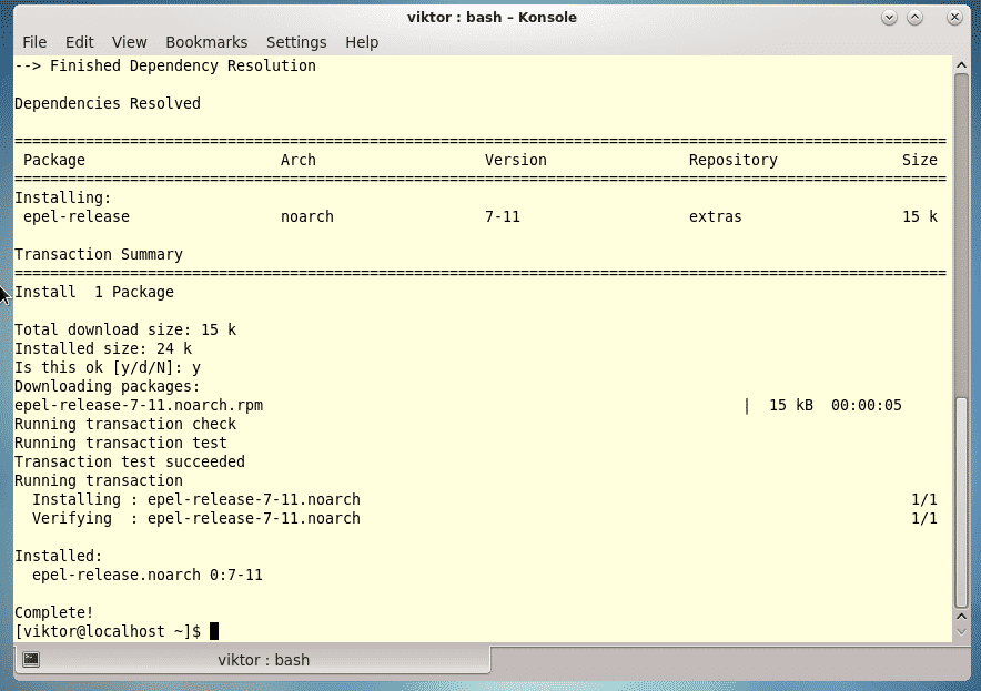
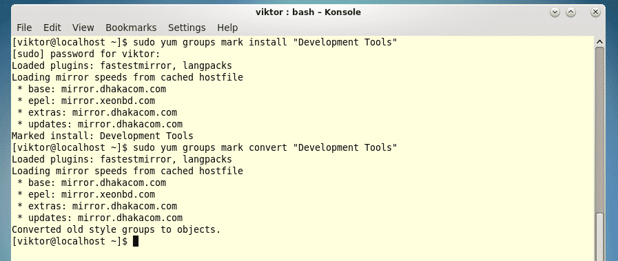
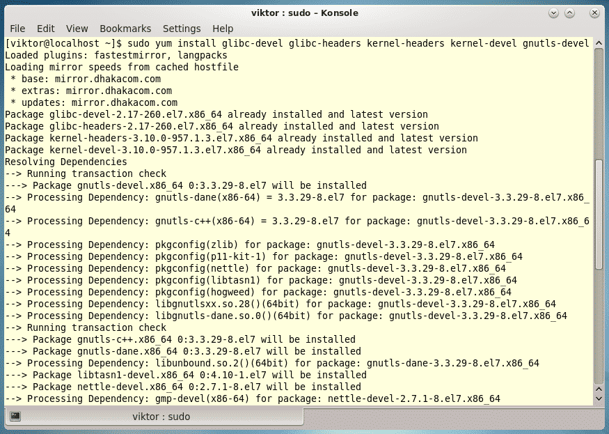
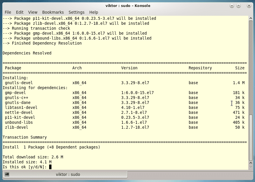
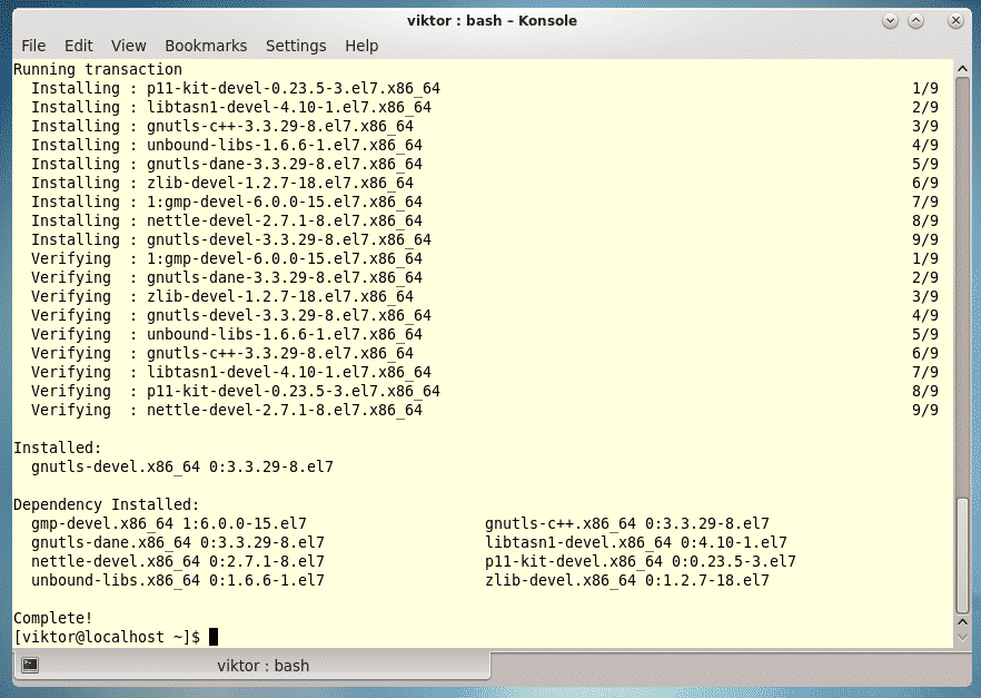
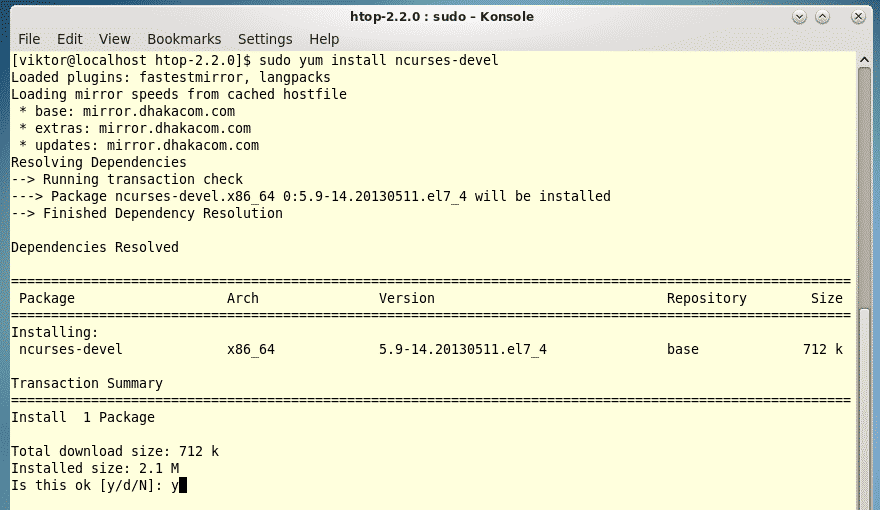
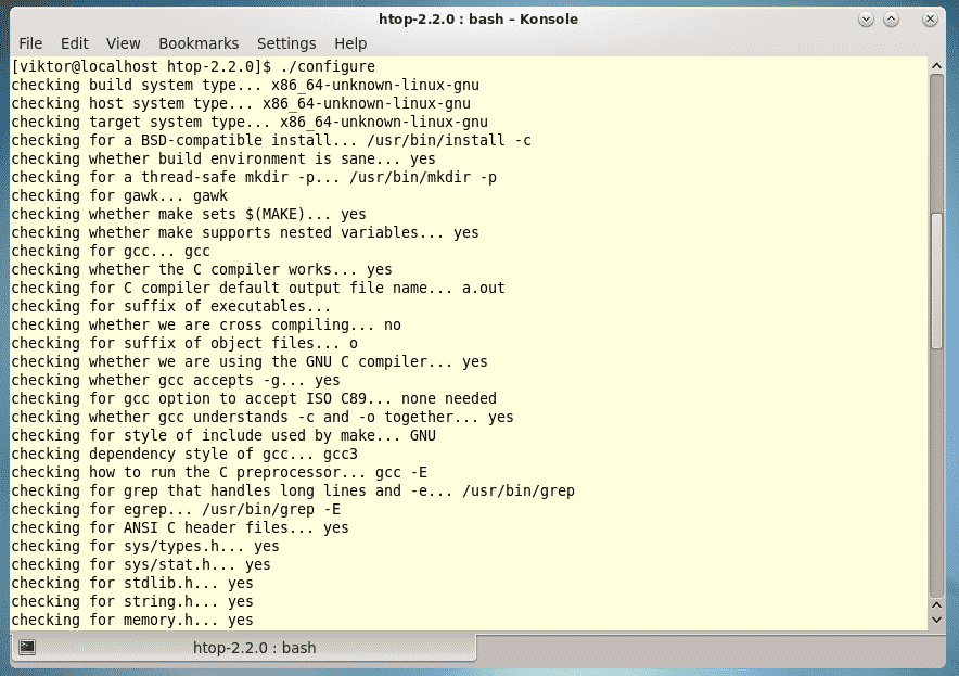
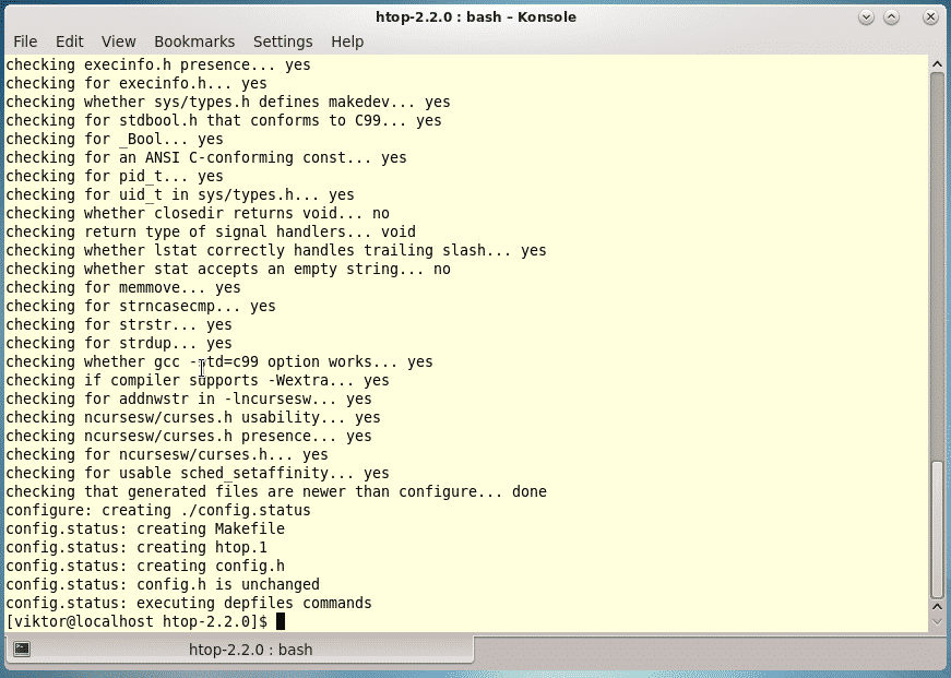
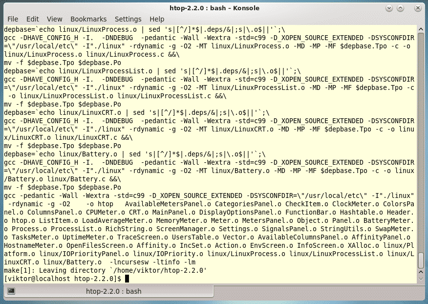
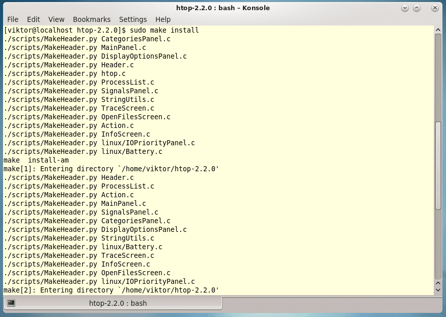
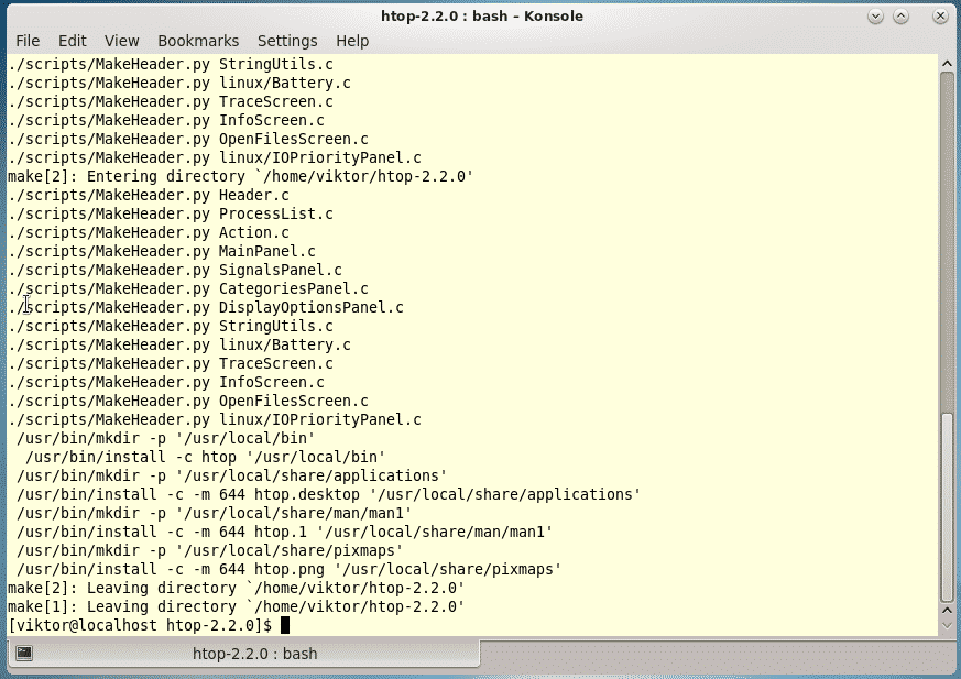
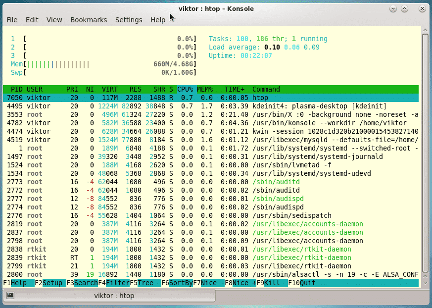
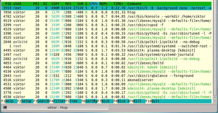
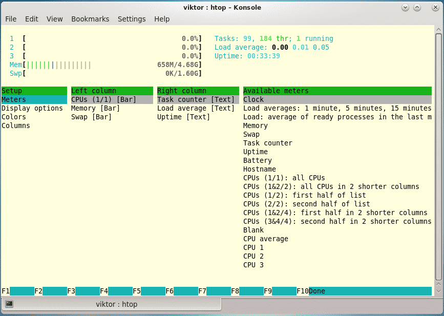
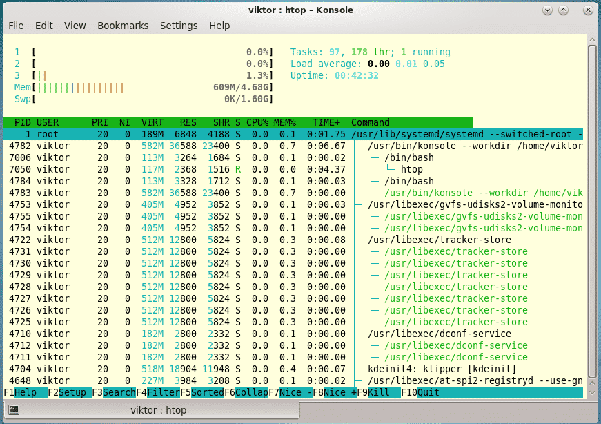
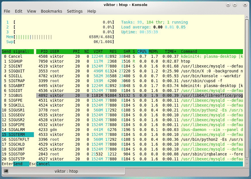
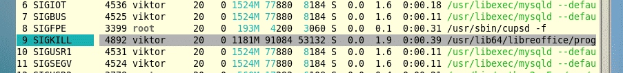
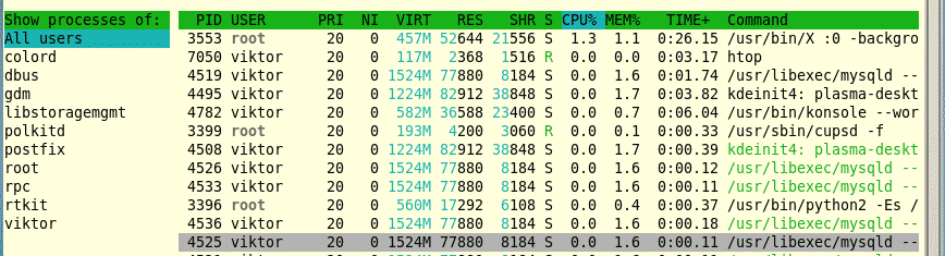
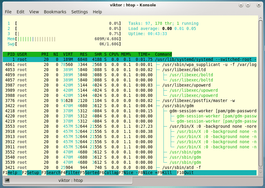
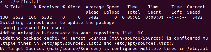
 How to install Java on CentOS 7