Zabbix is very popular, easy to use, fast monitoring tool. It support monitoring Linux, Unix, windows environments with agents, SNMP v1,v2c,c3, agentless remote monitoring. It can also monitor remote environment with a proxy without opening port for remote environments. You can send email, sms, IM message, run sny type of script to automate daily or emergency tasks based on any scenario.
Zabbix 4 is the latest version. New version supports php7, mysql 8, encryption between host and clients, new graphical layout, trend analysis and many more. With zabbix you can use zabbix_sender and zabbix_get tools to send any type of data to zabbix system and trigger alarm for any value. With these capabilities Zabbix is programmable and your monitoring is limited to your creativity and capability.
Installing from Zabbix repository is the easiest way. In order to setup from source file you need to setup compilers and make decisions about which directories and features get used for your environment. The Zabbix repository files provide all features enable and ready to go environment for your needs.
If you had the chance to use the setup we have select xfce for desktop environment. If you have not rest of the installation steps will perfectly work even if you had minimal setup environment which is the cleanest environment you find for Debian.

Security First!
Login to the root user and add the guest user to soders file simple adding.
Username ALL=(ALL:ALL) ALL
Into the configuration file /etc/sudoers
You can also use
To directly edit the file with the default text editor (nano in my case)


Install Mysql
Once you create the guest user and give root privileges we can login to the user with
and start to add sudo in front of the commands to send root commands with control.
Install Mysql with following command
$ sudo apt-get install mysql-server

Press ‘Y’ in order to download and install.

Right after the installation add mysql to the startup sequence so when system reboots your mysql server will be up.
$ sudo systemctl enable mariadb
$ sudo systemctl start mariadb

You can test if mysql is up with the following command
You should be able to login to the database server without entering a password.

Type quit to log out of the server

Install Zabbix from Repository
Once the database server installation has finished we can start installing zabbix application.
Download apt repo package to the system
$sudo wget https://repo.zabbix.com/zabbix/4.0/debian/pool/main/z/zabbix-release/zabbix-release_4.0-2+stretch_all.deb
$ sudo dpkg -i zabbix-release_4.0-2+stretch_all.deb
$sudo apt update
Lets install Zabbix server and front end packages.
$ sudo apt install zabbix-server-mysql zabbix-frontend-php zabbix-agent


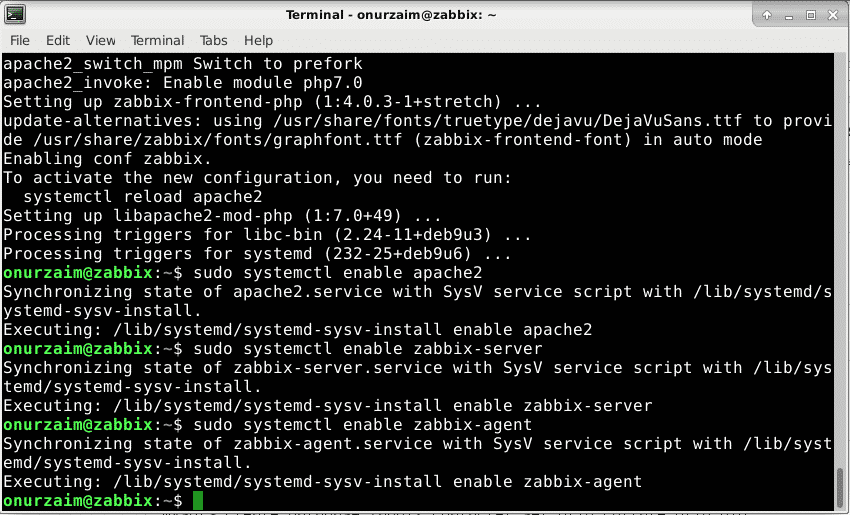
Add Zabbix Services to Startup
Once all packages are installed enable Zabbix services but don’t start yet. We need modifications on the configuration file.
$ sudo systemctl enable apache2
$ sudo systemctl enable zabbix-server
$ sudo systemctl enable zabbix-agent
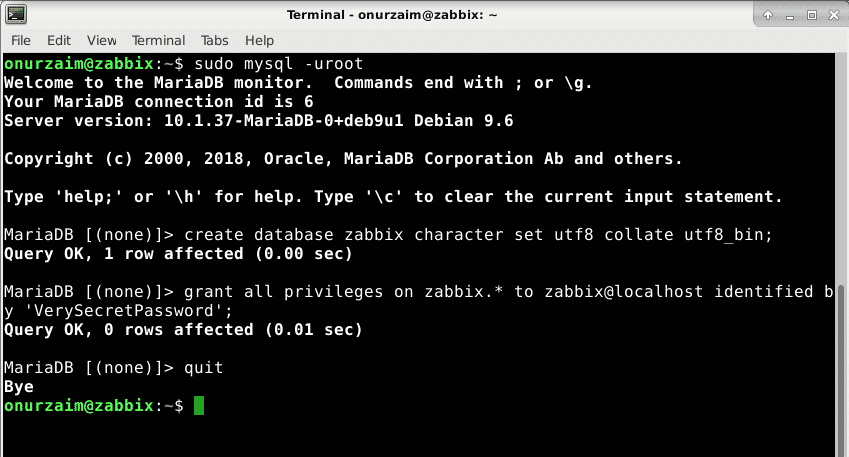
Create Database and Deploy Zabbix Database Tables
Now it is time to create database for Zabbix. Please note you can create a database with any name and a user. All you need is replace apropirate value with the commands we provided below.
In our case we will pickup (all are case sensitive)
We create zabbix database and user with mysql root user
After creating database and users we create the Zabbix database tables in our new database with the following command
# zcat /usr/share/doc/zabbix-server-mysql*/create.sql.gz | mysql -uzabbix -p -B Zabbix
Enter your database password in next step
Process may take about 1-10 minutes depending on your performance of server.

Configure Zabbix Server
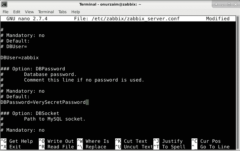
In order to have our Zabbix server start and get ready for business we must define database parameters into the zabbix_server.conf
$ sudo nano /etc/zabbix/zabbix_server.conf
DBHost=localhost
DBUser=zabbix
DBPassword=VerySecretPassword
DBName=zabbix
Time zone needs to be entered into /etc/zabbix/apache.conf file in order not to face any time related inconsistency in our environment. Also this step is a must for a errorless environment. If this parameter is not set Zabbix web interface will warn us every time. In my case the time zone is Europe/Istanbul.
You can get full list of PHP time zones here.
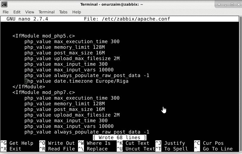
Please also note there are php7 and php5 segments here. In our setup php 7 was installed so modifying the php_value date.timezone in the php7.c segment was enough but we recommend modifying the php5 for compatibility issues.
Save the file.
Now stop and start services in order to have all changes in affect.
$ sudo systemctl restart apache2 zabbix-server zabbix-agent
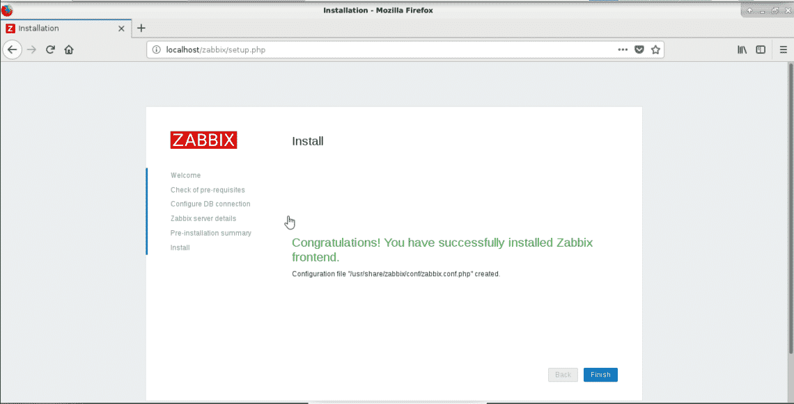
Setting up Web Server
Now database and Zabbix services are up. In order to check whats going in our systems we should setup web interface with mysql support. This is our last step before going online and start checking some stats.
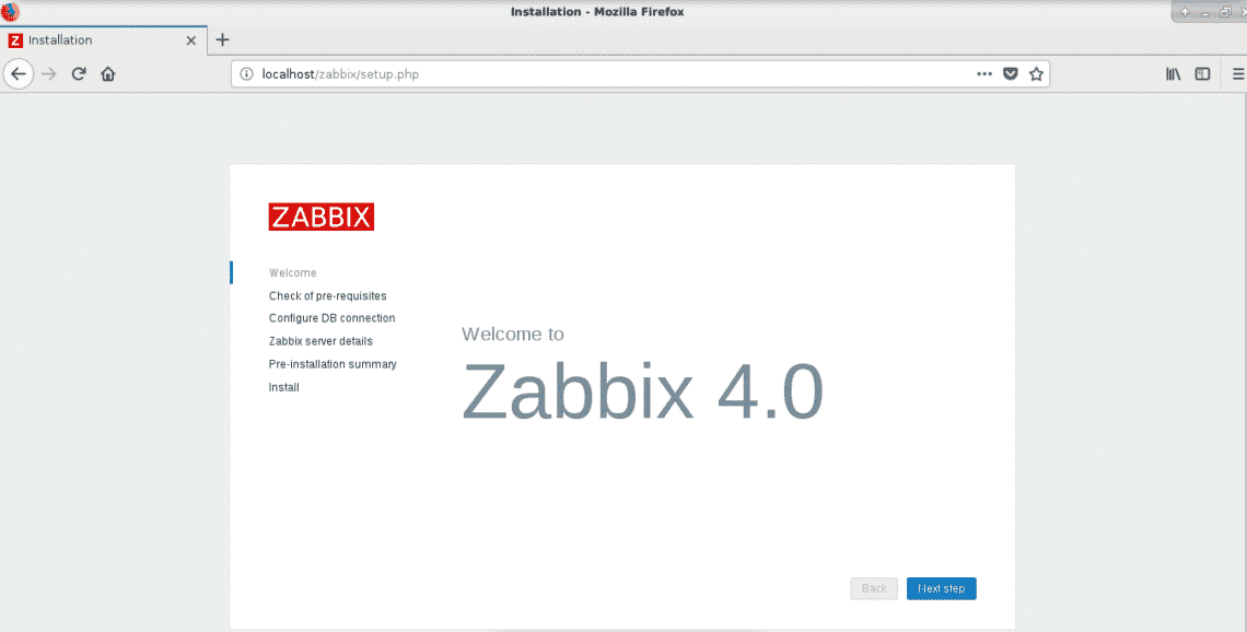
Welcome Screen.

Check if everything in ok with Green color.

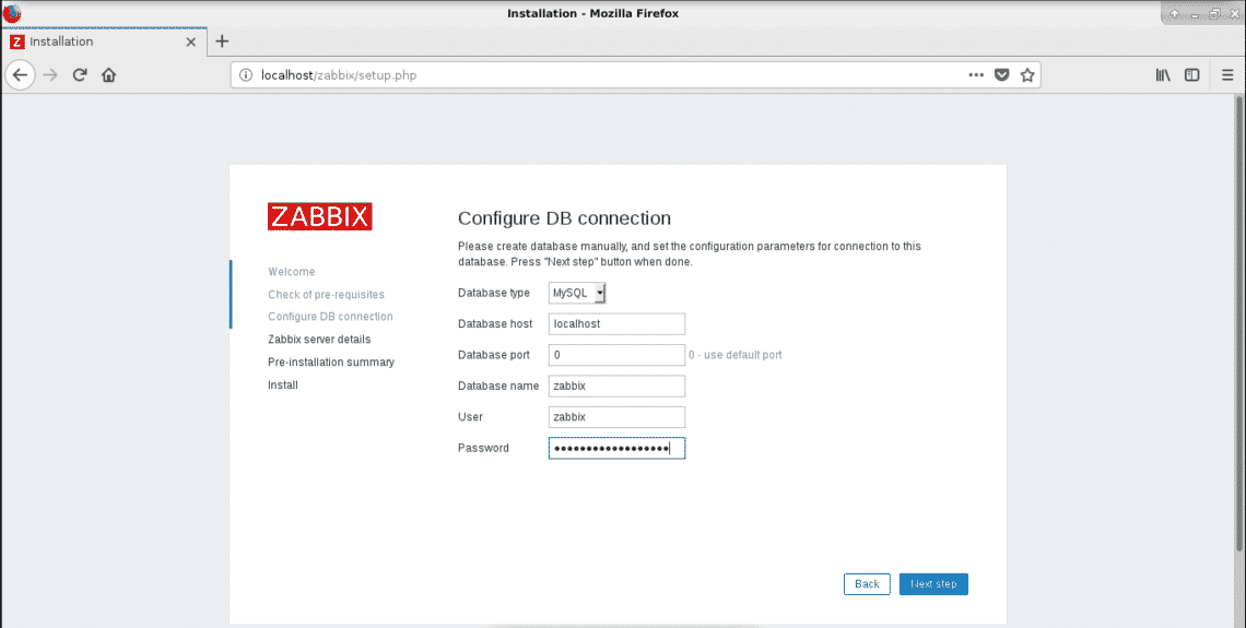
Define user name and password we defined in setting up database section.
DBHost=localhost
DBUser=zabbix
DBPassword=VerySecretPassword
DBName=zabbix
You can define Zabbix-server name in this step. You want to have it called something like watch tower or monitoring server something like it too.
Note: You can change this setting from
/etc/zabbix/web/zabbix.conf.php
You can change the $ZBX_SERVER_NAME parameter in the file.
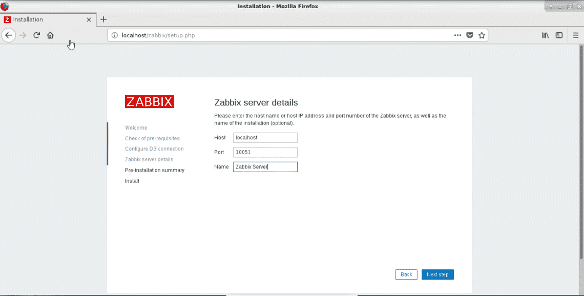
Verify setting and press Next Step

Default username and password are (case sensitive)

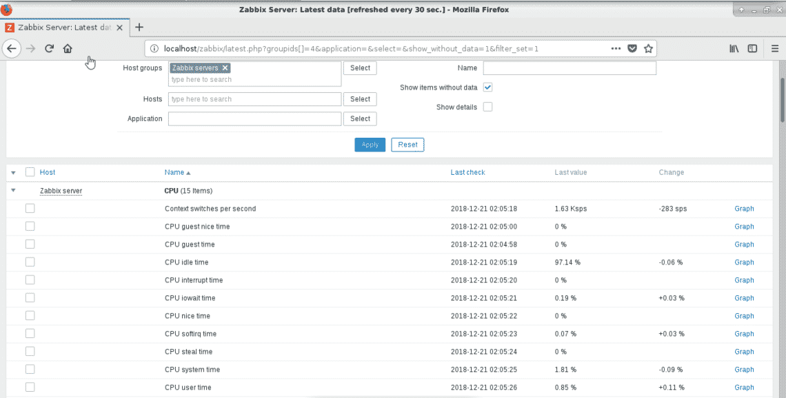
Now you can check your system stats.

Go to Monitoring -> Latest data
And select Zabbix Server from Host groups and check if stats are coming live.
Conclusion
We have setup the database server in the beginning because a system with already installed packages can prevent any version or mysql version we want to download because of conflicts. You can also download mysql server from the mysql.com site.
Later on we continued with Zabbix binary package installation and created database and user. Next step was to configure Zabbix configuration files and install web interface. In later stages you can install SSL, modify configuration for a specific web domain, proxy through nginx or directly run from nginx with php-fpm, upgrade PHP and such things like things. You may also disable Zabbix-agent in order to save from database space. It is all up to you.
Now you can enjoy monitoring with Zabbix. Have a Nice Day.
Source