The evolving landscape of API protocols in 2023

The API landscape is constantly evolving, with some protocols rising in popularity while others fade. Postman’s latest State of the API report, which is based on a survey of over 40,000 developers, offers a snapshot of these shifts—and reveals which API protocols are capturing the most attention and adoption right now. In this article, we’ll explore these API protocols in detail, analyze why they are attracting so much interest, and dive into the key strengths and limitations of each one.

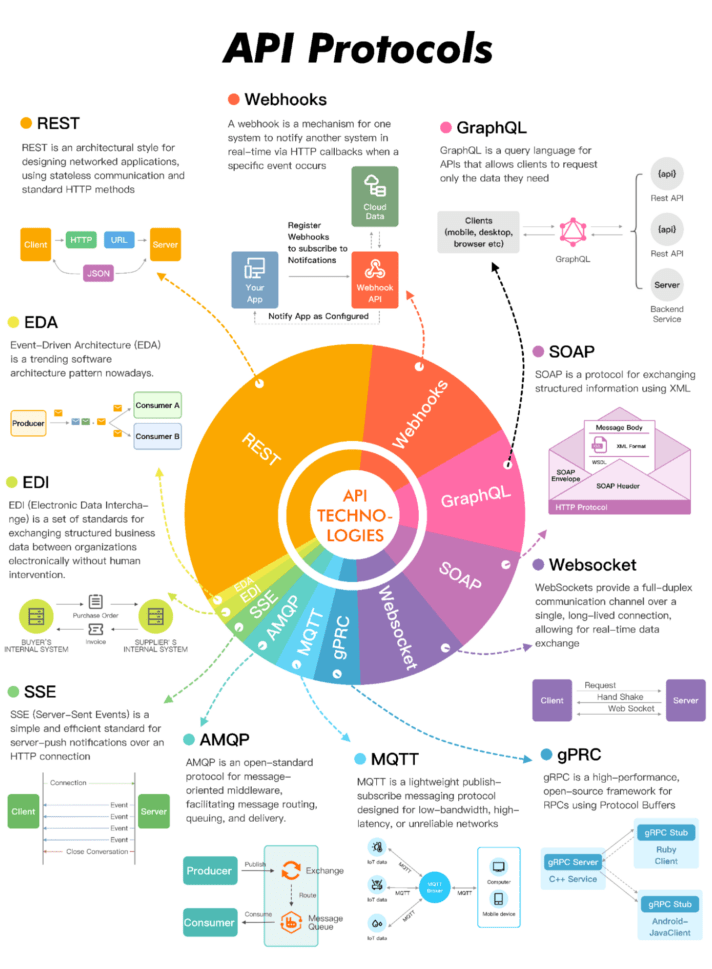
An overview of the API protocols in use today.
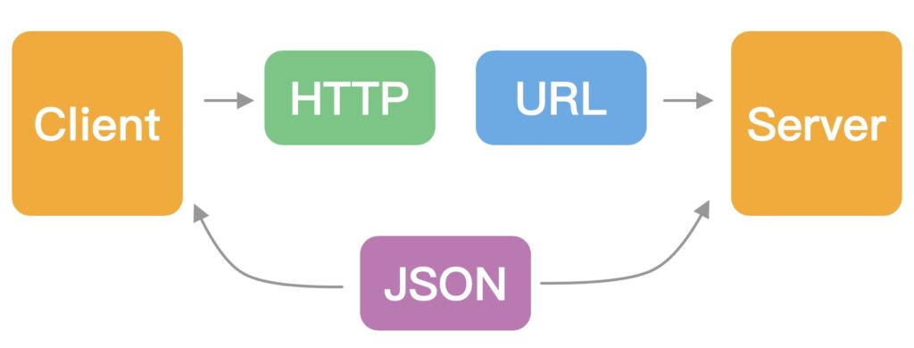
REST

Representational State Transfer (REST) remains the most popular architectural style for web APIs. Although its usage among survey respondents has declined slightly—from 92% to 86% over the past two years—its simplicity, scalability, and ease of integration with web services cement its position at the top.

A high-level look at RESTful architecture.

Benefits of REST

  • Simplicity and standardization: By leveraging standard HTTP methods, REST enables straightforward adoption for developers who are already versed in HTTP. This simplicity promotes rapid learning and integration.
  • Scalability: REST’s stateless nature ensures that servers do not need to store session data between requests. This facilitates horizontal scaling by adding instances without a shared server state.
  • Performance: Statelessness and cacheable responses yield faster execution and fewer requests.
  • Modularity: RESTful services can be developed as modular components. This localized functionality enables independent updates and improves maintainability.
  • Platform-agnostic: Platform-agnostic HTTP support allows for consumption by diverse clients. The resulting interoperability promotes API integration across systems.
  • Mature tooling and community support: REST’s longevity has led to the extensive proliferation of tools, libraries, best practices, troubleshooting guidance, and community resources.

Challenges of REST

  • Over-fetching and under-fetching: REST runs the risk of over-fetching or under-fetching data, as clients may only need a subset of resources. This drawback can cause performance issues and waste bandwidth.
  • Chatty interfaces: Retrieving related data may require multiple requests, which increases latency. This waterfall of calls becomes especially problematic as applications scale.
  • Versioning challenges: Creating new versions of a REST API can be cumbersome, especially when there are changes to the data structure or service functionality. This often leads to backward compatibility issues.
  • Stateless overhead: While statelessness supports scalability, it also means that all the necessary context must be provided with every request. This requirement can introduce overhead, especially when clients must send large amounts of repetitive data.
  • Lack of real-time functionality: REST is not optimized for real-time apps like chat or live feeds. WebSockets and Server-Sent Events often better suit such use cases.

Webhooks 

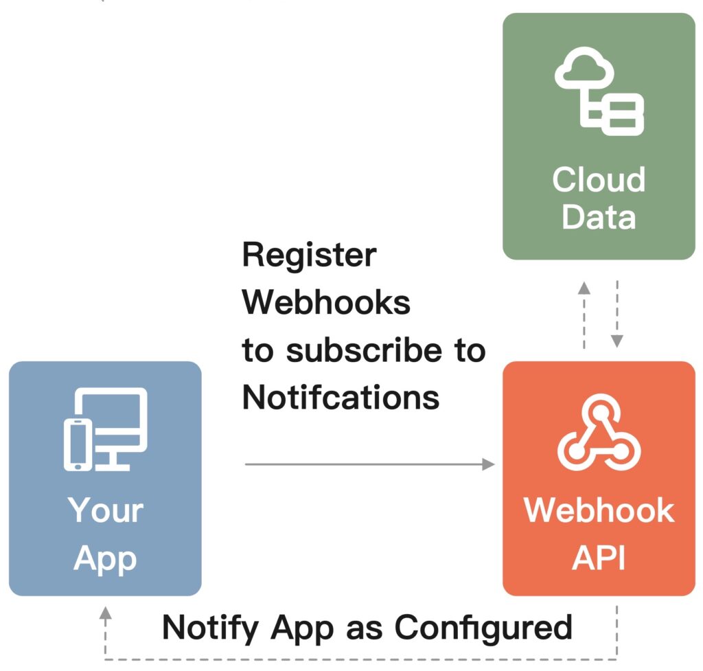
Webhooks are user-defined HTTP callbacks that are triggered by events in a source application. When an event occurs, the source application sends an HTTP request (usually POST) to a URI specified by the target application, which enables near real-time event-based communication without repeated polling. Webhooks are becoming increasingly popular, with 36% of developers using them to create seamless integrations between diverse systems.

For example, if you wanted to get notified every time there’s a new comment on your blog post, instead of repeatedly asking (polling) the server, “Is there a new comment?”, the server would notify you (via webhook) when a new comment has been posted.

Webhooks in action.

Benefits of webhooks

  • Real-time communication: Webhooks enable real-time data transmission. The corresponding data is sent when an event is triggered, ensuring up-to-date synchronization between systems.
  • Efficiency: Webhooks eliminate resource-intensive polling, saving computing power and bandwidth.
  • Flexibility: Webhooks can be configured to respond to specific events, allowing you to customize which actions or triggers in one application will send data to another.
  • Simplified integration: HTTP methods enable easy consumption by most applications.
  • Support for decoupled architectures: Since webhooks operate based on events, they naturally support event-driven or decoupled architectures, enhancing modularity and scalability.

Challenges of webhooks

  • Error handling: If the receiving end of a webhook is down or there’s an error in processing the callback, there’s a risk of data loss. Systems that use webhooks must have robust error-handling mechanisms, including retries or logs.
  • Security concerns: Webhooks transmit data over the internet, making them vulnerable to interceptions or malicious attacks. API security measures, such as the use of HTTPS and payload signatures, are essential.
  • Managing multiple webhooks: Managing and monitoring webhooks can be complex—especially as applications grow and begin to rely on multiple webhooks. Ensuring all webhooks function correctly and track various endpoints requires diligence.
  • Potential for overload: High volumes of concurrent callbacks can overwhelm receiving applications, but rate limiting or batching may help manage surges.

GraphQL

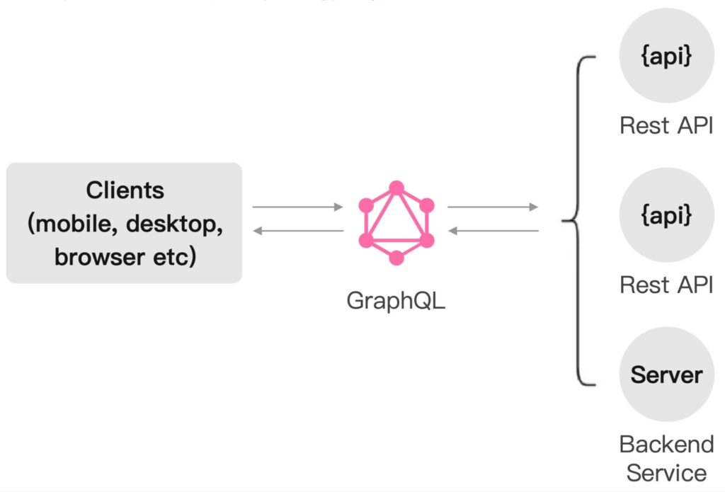
GraphQL is a query language for APIs and a server-side runtime for executing queries using a type system you define for your data. Developed by Facebook in 2012 and released as an open source project in 2015, GraphQL provides a more flexible and efficient alternative to the traditional REST API. GraphQL has a growing adoption rate of 29% among developers, indicating its importance in today’s API landscape.

Unlike REST, where you must hit multiple API endpoints to fetch related data, GraphQL lets you get all the data you need in a single query. This is particularly useful for frontend developers, as it gives them more control over the data retrieval process and allows them to create more dynamic and responsive user interfaces.

A high-level look at GraphQL’s architecture.

Benefits of GraphQL

  • Strongly typed schema: GraphQL APIs have strongly typed schemas, which allow developers to know exactly what data and types are available to query.
  • Precise data retrieval: Clients can request the precise data they need, which solves the problems of over-fetching and under-fetching and, by extension, improves performance and lowers costs.
  • Query complexity and multiple resources: GraphQL supports querying multiple data types in one request, which reduces the number of network requests for complex, inter-related data.
  • Real-time updates with subscriptions: GraphQL enables real-time syncing through subscriptions, which keep the client updated in real time.
  • Introspection: GraphQL’s self-documenting schema enables easier development through introspection.

Challenges of GraphQL

  • Query complexity: The flexibility that GraphQL gives to the client comes with drawbacks, as overly complex or nested queries can negatively impact performance.
  • Learning curve: GraphQL has a steeper learning curve than REST due to new concepts like mutations and subscriptions.
  • Versioning: The flexible nature of queries means that changes in the schema can break existing queries, complicating version management.
  • Potential overuse of resources: Since clients can request multiple resources in one query, there’s a risk of overloading servers by fetching more data than necessary.
  • Security concerns: Malicious users could exploit GraphQL’s flexibility to overload servers with complex queries.

SOAP 

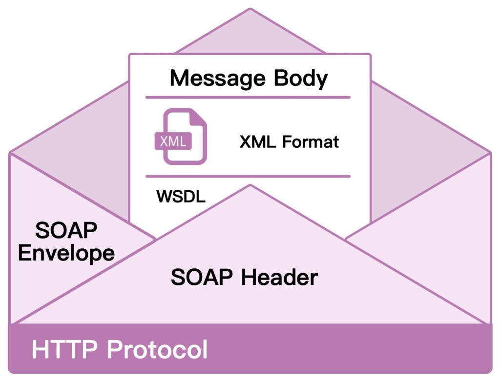
Simple Object Access Protocol (SOAP) is a protocol for exchanging structured information to implement web services. It uses XML for its message format and usually employs HTTP or SMTP as the message negotiation and transmission layer. Unlike REST and GraphQL, SOAP has strict standards and built-in features like ACID-compliant transactions, security, and messaging patterns.

Despite its reduced usage—down to just 26% of developers—SOAP is a reliable choice for certain applications. Let’s explore what makes SOAP unique and where it shines compared to other API design approaches.

A SOAP envelope.

Benefits of SOAP

  • Strong typing and contracts: SOAP APIs have strong typing and a strict contract that is defined in a Web Services Description Language (WDSL) document.
  • Built-in security features: SOAP provides comprehensive security with authentication, authorization, and encryption baked in via the WS-Security standard. This makes SOAP a preferred choice for enterprise applications.
  • ACID transactions: SOAP supports ACID transactions, which are essential for applications where data integrity is crucial, such as financial or healthcare systems.
  • Reliable messaging: SOAP ensures reliable message delivery and handles failures well, which makes it a great fit for systems in which guaranteed message delivery is critical.
  • Language, platform, and transport neutrality: Similar to REST, SOAP services can be consumed by any client that understands XML, regardless of its underlying programming language, platform, or transport protocol.

Challenges of SOAP

  • Complexity and learning curve: SOAP can be more complex to implement due to its strict standards and use of XML, making the learning curve steeper than that of alternatives like REST or GraphQL.
  • Verbose messages: SOAP message headers carry a lot of overhead, which results in larger payloads than in REST and GraphQL’s JSON. This can affect performance and bandwidth usage.
  • Limited community support: SOAP is losing ground, which means that community support and available libraries are declining.
  • Less flexibility: Any change in the contract may require both the client and server to update their respective implementations, which can be a downside.
  • Firewall issues: SOAP may use different transport protocols than HTTP/HTTPS, which means it can face firewall restrictions. This makes SOAP less versatile for some deployment environments.

WebSocket 

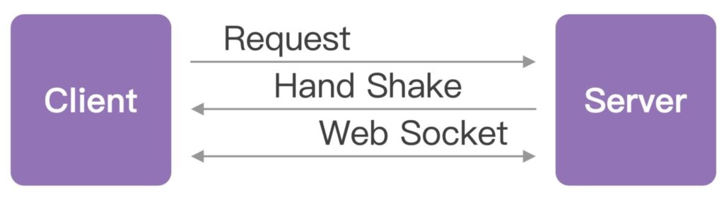
WebSocket provides a persistent, low-latency, bidirectional connection between client and server, enabling real-time data transfer. Unlike HTTP’s request-response cycle, WebSocket allows the server to send data to clients any time after the initial handshake. This facilitates instant data updates for chat applications, online games, trading platforms, and more.

Survey results indicate that 25% of developers use WebSocket. Let’s explore its advantages, challenges, and use cases.

Benefits of WebSocket

  • Real-time bidirectional communication: Real-time bidirectional communication has less latency than HTTP connections that must be re-established for each exchange.
  • Lower overhead: The connection remains open after the initial handshake, which lowers the overhead of headers that come with traditional HTTP requests.
  • Efficient use of resources: Persistent connections use server resources more efficiently than long polling.

Challenges of WebSocket

  • Implementation complexityImplementing WebSocket can be more complex and time-consuming than other API architectures—especially when you take into account the need for fallbacks in environments where WebSocket is not supported.
  • Lack of built-in featuresUnlike SOAP, which comes with built-in features for security and transactions, WebSocket is more bare-bones. It requires developers to implement these features themselves.
  • Resource consumptionAlthough open WebSocket connections are generally more efficient than long-polling techniques, they still consume server resources and can become a concern at scale.
  • Network limitationsSome proxies and firewalls do not support WebSocket, leading to potential connectivity issues in certain network environments.

gRPC

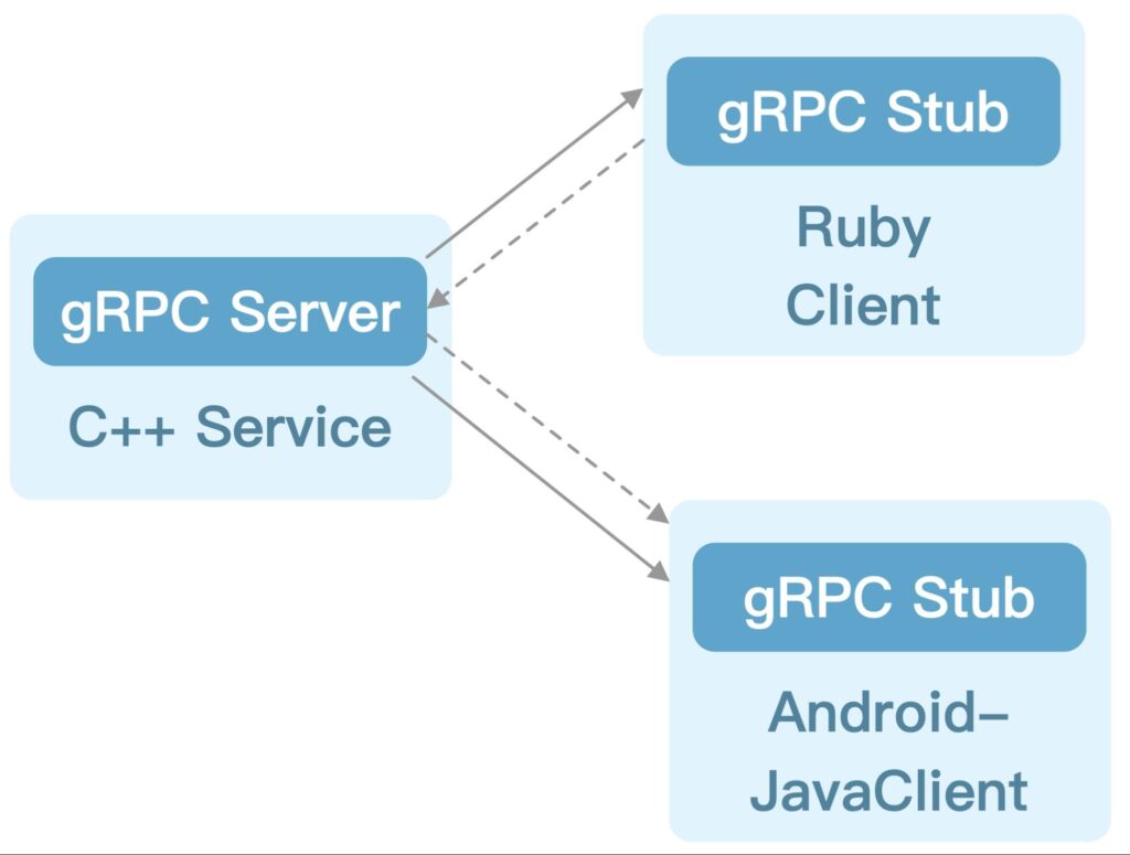
gRPC, which stands for “Google Remote Procedure Call,” is a modern, high-performance protocol that facilitates communication between services. It is built on top of HTTP/2 and leverages Protocol Buffers to define service methods and message formats. In contrast to REST APIs, which rely on standard HTTP verbs like GET and POST, gRPC enables services to expose custom methods that are similar to functions in a programming language.

gRPC facilitates communication between distributed services in different programming languages.

Benefits of gRPC

  • Performance: HTTP/2 and Protocol Buffers enable gRPC to achieve low latency and high throughput.
  • Strong typing: Like SOAP and GraphQL, gRPC is strongly typed. This results in fewer bugs as types are validated at compile time.
  • Multi-language support: gRPC has first-class support for many programming languages, including Go, Java, C#, and Node.js.
  • Streaming: gRPC handles streaming requests and responses out-of-the-box, which unlocks complex use cases like long-lived connections and real-time updates.
  • Battery included: gRPC directly supports critical functionality like load balancing, retries, and timeouts.

Challenges of gRPC

  • Browser support: Native gRPC support in browsers is still limited, making it less suitable for direct client-to-server communication in web applications.
  • Learning curve: Developers need to learn how to work with Protocol Buffers, custom service definitions, and other gRPC features, which can slow initial productivity.
  • Debugging complexity: Protocol Buffers are not human-readable, making it harder to debug and test gRPC APIs than JSON APIs.

Other API protocols

While the previously discussed protocols are the most widely adopted in the API landscape today, Postman’s State of the API report also highlights a few other approaches that serve specific use cases:

  • MQTT is a lightweight messaging protocol optimized for low-bandwidth networks like IoT. It allows clients to publish and subscribe to messages through a broker, but it lacks some security and scalability features.
  • AMQP is a more robust enterprise messaging standard that ensures reliable delivery and flexible routing of messages. However, it can be complex and has more overhead than lightweight protocols.
  • SSE enables uni-directional server-to-client communication over HTTP. It is great for real-time updates, but it lacks bidirectional capabilities.
  • EDI automates B2B communications by standardizing electronic documents like purchase orders and invoices, but it also requires complex infrastructure with high initial costs.
  • EDA promotes an event-driven architecture where components react to events, enabling real-time systems that are scalable yet complex to debug.

These protocols are not as ubiquitous, but they enable specialized applications in IoT, enterprise messaging, B2B transactions, and event-driven systems. By selecting the right approach for their specific needs, developers can build optimized API solutions that go beyond the common standards.

Conclusion

The API landscape continues to evolve as developers adopt new architectures, protocols, and tools. While REST remains dominant due to its simplicity and ubiquity, alternatives like GraphQL and gRPC are gaining traction by solving pain points like over-fetching and chatty interfaces. Developers are also increasingly valuing real-time communication, with webhooks and WebSockets rising to meet this demand.

For many common API use cases, REST remains a solid foundational approach given its scalability, interoperability, and ease of adoption. It also still benefits from community maturity. Still, every protocol presents trade-offs, and as applications grow more complex, developers are wisely expanding their API protocol toolkit to include specialized solutions like GraphQL and gRPC.

Rather than a one-size-fits-all panacea, the modern API developer is best served by understanding the strengths and weaknesses of multiple protocols. By architecting systems that combine REST, webhooks, WebSockets, GraphQL, and other approaches where each uniquely shines, developers can build robust, efficient, and maintainable APIs. While the popularity of individual protocols will continue to fluctuate, the overarching trend is towards increased diversity in the API landscape. Developers should embrace this multi-protocol philosophy to craft optimal API solutions.

Source

Native Kubernetes Monitoring: Monitoring and Metrics for Users


Introduction

Kubernetes is an open-source orchestration platform for working with containers. At its core, it gives us the means to do deployments, easy ways to scale, and monitoring. In this article, we will talk about the built-in monitoring capabilities of Kubernetes and include some demos for better understanding.

Brief Overview of Kubernetes Architecture

At the infrastructure level, a Kubernetes cluster is a set of physical or virtual machines, each acting in a specific role. The machines acting in the role of master function as the brain of the operations and are charged with orchestrating the management of all containers that run on all of the nodes.

  • Master components manage the life cycle of a pod:
    • apiserver: main component exposing APIs for all the other master components
    • scheduler: uses information in the pod spec to decide on which node to run a pod
    • controller-manager: responsible for node management (detecting if a node fails), pod replication, and endpoint creation
    • etcd: key/value store used for storing all internal cluster data
  • Node components are worker machines in Kubernetes, managed by the master. Each node contains the necessary components to run pods:
    • kubelet: handles all communication between the master and the node on which it is running. It interfaces with the container runtime to deploy and monitor containers
    • kube-proxy: is in charge with maintaining network rules for the node. It also handles communication between pods, nodes, and the outside world.
    • container runtime: runs containers on the node.

From a logical perspective, a Kubernetes deployment is comprised of various components, each serving a specific purpose within the cluster:

  • Pods: are the basic unit of deployment within Kubernetes. A pod consists of one or more containers that share the same network namespace and IP address.
  • Services: act like a load balancer. They provide an IP address in front of a pool (set of pods) and also a policy that controls access to them.
  • ReplicaSets: are controlled by deployments and ensure that the desired number of pods for that deployment are running.
  • Namespaces: define a logical segregation for different kind of resources like pods and/or services.
  • Metadata: marks containers based on their deployment characteristics.

Monitoring Kubernetes

Monitoring an application is absolutely required if we want to anticipate problems and have visibility of potential bottlenecks in a dev or production deployment.

To help monitor the cluster and the many moving parts that form a deployment, Kubernetes ships with some built-in monitoring capabilities:

  • Kubernetes dashboard: gives an overview of the resources running on your cluster. It also gives a very basic means of deploying and interacting with those resources.
  • cAdvisor: is an open source agent that monitors resource usage and analyzes the performance of containers.
  • Liveness and Readiness Probes: actively monitor the health of a container.
  • Horizontal Pod Autoscaler: increases the number of pods if needed based on information gathered by analyzing different metrics.

In this article, we will be covering the first two built-in tools. A follow up article focusing on the remaining tools can be found here.

There are many Kubernetes metrics to monitor. As we’ve described the architecture in two separate ways (infrastructure and logical), we can do the same with monitoring and separate this into two main components: monitoring the cluster itself and monitoring the workloads running on it.

Cluster Monitoring

All clusters should monitor the underlying server components since problems at the server level will show up in the workloads. Some metrics to look for while monitoring node resources are CPU, disk, and network bandwidth. Having an overview of these metrics will let you know if it’s time to scale the cluster up or down (this is especially useful when using cloud providers where running cost is important).

Workload Monitoring

Metrics related to deployments and their pods should be taken into consideration here. Checking the number of pods a deployment has at a moment compared to its desired state can be relevant. Also, we can look for health checks, container metrics, and finally application metrics.

Prerequisites for the Demo

In the following sections, we will take each of the listed built-in monitoring features one-by-one to see how they can help us. The prerequisites needed for this exercise include:

  • a Google Cloud Platform account: the free tier is more than enough. Most other cloud should also work the same.
  • a host where Rancher will be running: This can be a personal PC/Mac or a VM in a public cloud.
  • Google Cloud SDK: should be installed along kubectl on the host running Rancher. Make sure that gcloud has access to your Google Cloud account by authenticating with your credentials (gcloud init and gcloud auth login).

Starting a Rancher Instance

To begin, start your Rancher instance. There is a very intuitive getting started guide for Rancher that you can follow for this purpose.

Using Rancher to Deploy a GKE cluster

Use Rancher to set up and configure a Kubernetes cluster by following the how-to guide.

As mentioned previously, in this guide we will be covering the first two built-in tools: the Kubernetes dashboard and cAdvisor. A follow up article that discusses probes and horizontal pod autoscalers can be found here.

Kubernetes Dashboard

The Kubernetes dashboard is a web-based Kubernetes user interface that we can use to troubleshoot applications and manage cluster resources.

Rancher, as seen above, helps us install the dashboard by just checking a radio button. Let’s take a look now at how the dashboard can help us by listing some of its uses:

  • Provides an overview of cluster resources (overall and per individual node), shows us all of the namespaces, lists all of the storage classes defined
  • Shows all applications running on the cluster
  • Provides information about the state of Kubernetes resources in your cluster and on any errors that may have occurred

To access the dashboard, we need to proxy the request between our machine and Kubernetes API server. Start a proxy server with kubectl by typing the following:

kubectl proxy &

The proxy server will start in the background, providing output that looks similar to this:

[1] 3190
$ Starting to serve on 127.0.0.1:8001

Now, to view the dashboard, navigate to the following address in the browser:

http://localhost:8001/api/v1/namespaces/kube-system/services/https:kubernetes-dashboard:/proxy/

We will then be prompted with the login page to enter the credentials:

Fig. 4: Dashboard login

Fig. 4: Dashboard login

Let’s take a look on how to create a user with admin permission using the Service Account mechanism. We will use two YAML files.

One will create the Service Account:

cat ServiceAccount.yaml
apiVersion: v1
kind: ServiceAccount
metadata:
  name: admin-user
  namespace: kube-system

The other will create the ClusterRoleBinding for our user:

cat ClusterRoleBinding.yaml
apiVersion: rbac.authorization.k8s.io/v1
kind: ClusterRoleBinding
metadata:
  name: admin-user
roleRef:
  apiGroup: rbac.authorization.k8s.io
  kind: ClusterRole
  name: cluster-admin
subjects:
- kind: ServiceAccount
  name: admin-user
  namespace: kube-system

Apply the two YAML files to create the objects they define:

kubectl apply -f ServiceAccount.yaml 
kubectl apply -f ClusterRoleBinding.yaml 
serviceaccount "admin-user" created
clusterrolebinding.rbac.authorization.k8s.io "admin-user" created

Once our user is created and the correct permissions have been set, we will need to find out the token in order to login:

kubectl -n kube-system describe secret $(kubectl -n kube-system get secret | grep admin-user | awk '{print $1}')
Name:         admin-user-token-lnnsn
Namespace:    kube-system
Labels:       <none>
Annotations:  kubernetes.io/service-account.name=admin-user
              kubernetes.io/service-account.uid=e34a9438-4e12-11e9-a57b-42010aa4009e

Type:  kubernetes.io/service-account-token

Data
====
ca.crt:     1119 bytes
namespace:  11 bytes
token:      COPY_THIS_STRING

Select “Token” at the Kubernetes dashboard credentials prompt and enter the value you retrieved above in the token field to authenticate.

The Kubernetes Dashboard consists of few main views:

  • Admin view: lists nodes, namespaces, and persistent volumes along with other details. We can get an aggregated view for our nodes (CPU and memory usage metrics) and an individual details view for each node showing its metrics, specification, status, allocated resources, events, and pods.
  • Workload view: shows all applications running in a selected namespace. It summarizes important information about workloads, like the number of pods ready in a StatefulSet or Deployment or the current memory usage for a pod.
  • Discover and Load Balancing view: shows Kubernetes resources that expose services to the external world and enable discovery within the cluster.
  • Config and storage view: shows persistent volume claim resources used by applications. Config view is used to shows all of the Kubernetes resources used for live configuration of applications running in the cluster.

Without any workloads running, the dashboard’s views will be mainly empty since there will be nothing deployed on top of Kubernetes. If you want to explore all of the views the dashboard has to offer, the best option is to deploy apps that use different workload types (stateful set, deployments, replica sets, etc.). You can check out this article on deploying a Redis cluster for an example that deploys a Redis cluster (a stateful set with volume claims and configMaps) and a testing app (a Kubernetes deployment) so the dashboard tabs will have some relevant info.

After provisioning some workloads, we can take down one node and then check the different tabs to see some updates:

kubectl delete pod redis-cluster-2
kubectl get pods
pod "redis-cluster-2" deleted
NAME                              READY     STATUS        RESTARTS   AGE
hit-counter-app-9c5d54b99-xv5hj   1/1       Running       0          1h
redis-cluster-0                   1/1       Running       0          1h
redis-cluster-1                   1/1       Running       0          1h
redis-cluster-2                   0/1       Terminating   0          1h
redis-cluster-3                   1/1       Running       0          44s
redis-cluster-4                   1/1       Running       0          1h
redis-cluster-5                   1/1       Running       0          1h

cAdvisor

cAdvisor is an open-source agent integrated into the kubelet binary that monitors resource usage and analyzes the performance of containers. It collects statistics about the CPU, memory, file, and network usage for all containers running on a given node (it does not operate at the pod level). In addition to core metrics, it also monitors events as well. Metrics can be accessed directly, using commands like kubectl top or used by the scheduler to perform orchestration (for example with autoscaling).

Note that cAdvisor doesn’t store metrics for long-term use, so if you want that functionality, you’ll need to look for a dedicated monitoring tool.

cAdvisor’s UI has been marked deprecated as of Kubernetes version 1.10 and the interface is scheduled to be completely removed in version 1.12. Rancher gives you the option to choose what version of Kubernetes to use for your clusters. When setting up the infrastructure for this demo, we configured the cluster to use version 1.10, so we should still have access to the cAdvisor UI.

To access the cAdvisor UI, we need to proxy between our machine and Kubernetes API server. Start a local instance of the proxy server by typing:

kubectl proxy &
[1] 3190
$ Starting to serve on 127.0.0.1:8001

Next, find the name of your nodes:

kubectl get nodes

You can view the UI in you browser by navigating to the following address, replacing the node name with the identifier you found on the command line:

http://localhost:8001/api/v1/nodes/gke-c-plnf4-default-pool-5eb56043-23p5:4194/proxy/containers/

To confirm that kubelet is listening on port 4194, you can log into the node to get more information:

gcloud compute ssh admin@gke-c-plnf4-default-pool-5eb56043-23p5 --zone europe-west4-c
Welcome to Kubernetes v1.10.12-gke.7!

You can find documentation for Kubernetes at:
  http://docs.kubernetes.io/

The source for this release can be found at:
  /home/kubernetes/kubernetes-src.tar.gz
Or you can download it at:
  https://storage.googleapis.com/kubernetes-release-gke/release/v1.10.12-gke.7/kubernetes-src.tar.gz

It is based on the Kubernetes source at:
  https://github.com/kubernetes/kubernetes/tree/v1.10.12-gke.7

For Kubernetes copyright and licensing information, see:
  /home/kubernetes/LICENSES

We can confirm that in our version of Kubernetes, the kubelet process is serving the cAdvisor web UI over that port:

sudo su -
netstat -anp | grep LISTEN | grep 4194
tcp6       0      0 :::4194                 :::*                    LISTEN      1060/kubelet 

If you run Kubernetes version 1.12 or later, the UI has been removed, so kubelet does not listening on port 4194 anymore. You can confirm this with the commands above. However, the metrics are still there since cAdvisor is part of the kubelet binary.

The kubelet binary exposes all of its runtime metrics and all of the cAdvisor metrics at the /metrics endpoint using the Prometheus exposition format:

http://localhost:8001/api/v1/nodes/gke-c-plnf4-default-pool-5eb56043-23p5/proxy/metrics/cadvisor

Among the output, metrics you can look for include:

  • CPU:
    • container_cpu_user_seconds_total: Cumulative “user” CPU time consumed in seconds
    • container_cpu_system_seconds_total: Cumulative “system” CPU time consumed in seconds
    • container_cpu_usage_seconds_total: Cumulative CPU time consumed in seconds (sum of the above)
  • Memory:
    • container_memory_cache: Number of bytes of page cache memory
    • container_memory_swap: Container swap usage in bytes
    • container_memory_usage_bytes: Current memory usage in bytes, including all memory regardless of when it was accessed
    • container_memory_max_usage_bytes: Maximum memory usage in byte
  • Disk:
    • container_fs_io_time_seconds_total: Count of seconds spent doing I/Os
    • container_fs_io_time_weighted_seconds_total: Cumulative weighted I/O time in seconds
    • container_fs_writes_bytes_total: Cumulative count of bytes written
    • container_fs_reads_bytes_total: Cumulative count of bytes read
  • Network:
    • container_network_receive_bytes_total: Cumulative count of bytes received
    • container_network_receive_errors_total: Cumulative count of errors encountered while receiving
    • container_network_transmit_bytes_total: Cumulative count of bytes transmitted
    • container_network_transmit_errors_total: Cumulative count of errors encountered while transmitting

Some additional useful metrics can be found here:

  • /healthz: Endpoint for determining whether cAdvisor is healthy
  • /healthz/ping: To check connectivity to etcd
  • /spec: Endpoint returns the cAdvisor MachineInfo()

For example, to see the cAdvisor MachineInfo(), we could visit:

http://localhost:8001/api/v1/nodes/gke-c-plnf4-default-pool-5eb56043-23p5:10255/proxy/spec/

The pods endpoint provides the same output as kubectl get pods -o json for the pods running on the node:

http://localhost:8001/api/v1/nodes/gke-c-plnf4-default-pool-5eb56043-23p5:10255/proxy/pods/

Similarly, logs can also be retrieved by visiting:

http://localhost:8001/logs/kube-apiserver.log

Conclusion

Monitoring is vital in order to understand what is happening with our applications. Kubernetes helps us with a number of built-in tools and provides some great insights for both, infrastructure layer (nodes) and logical one (pods).

This article concentrated on the tools that focus on providing monitoring and metrics for users. Continue on to the second part of this series to learn about the included monitoring tools focused on workload scaling and life cycle management.

Source

HTTP Alternative RSocket Gets a Home at The Linux Foundation

The list of foundations hosted by the Linux Foundation continues growing this week with the launch of the Reactive Foundation, “a community of leaders established to accelerate technologies for building the next generation of networked applications,” according to a statement. Upon founding, those leaders will include Alibaba, Facebook, Netifi and Pivotal, with the open source RSocket specification and programming language implementations also joining the new foundation’s “formal open governance model and neutral ecosystem.”

RSocket provides a basis for reactive programming at the protocol level and lays the groundwork for reactive programming in cloud native environments, Ryland Degnan, co-founder and CTO at Netifi, said in an interview with The New Stack. It’s considered a replacement for HTTP in cloud native communications.

Lest you confuse reactive programming with the React UI Javascript framework of a similar name, reactive programming is defined by its message-driven approach that aims to achieve resiliency and scalability independent of infrastructure, network issues or end-user device. More specifically, the reactive manifesto lists four characteristics of reactive systems: responsive, resilient, elastic and message-driven.

“With the whole cloud native movement, a lot more people are building software for the cloud that operates on a scale that’s an order of magnitude higher than anything we’ve seen before. It’s got a lot of moving parts and rationalizing how all those parts communicate is an incredibly important problem,” Degnan said. “The present problem that RSocket is seeking to solve is defining a standardized way for services to communicate that was built from the ground up and not using last year’s technology.”

“The de facto standard right now when people go out and build stuff is to use HTTP. That comes with loads of problems because it was really designed to be a request-response protocol,” Degnan said. “It has very little that was built for microservices. It was really built for this previous generation of requesting a resource from a monolithic server and returning a response. RSocket has been designed from the ground up for cloud native communication.”

HTTP vs. RSocket

Originally created by Netflix, RSocket is an application protocol for Reactive Streams that provides application flow control over the network to prevent outages and increase resiliency. As opposed to HTTP, RSocket does not await a response or request from the client. Degnan explains this core difference between HTTP and RSocket.

“A lot of effort spent in building these distributed systems ends up being workarounds for problems with HTTP. Circuit breakers are a great example of that. It’s working around the problem that HTTP doesn’t have flow control built into it, which means that you have to guess whether the downstream service is available or not, to not cause it to receive too many requests,” said Degnan. “You need to cut off traffic to it if you think that it’s now unavailable, but that involves a lot of configurations. RSocket could remove that problem entirely.”

By contrast, RSocket employs the idea of asynchronous stream processing with non-blocking back-pressure, in which a failing component will, rather than simply dropping traffic, communicate its stress to upstream components, getting them to reduce the load and allowing the system to “gracefully respond to load rather than collapse under it,” according to the Reactive Manifesto glossary. Degnan further explained how this applied to the modern world of microservices.

“Reactive streams are designed to have vendors and receivers of information that are decoupled from each other. Rather than having the receiver control the flow of information, it’s allowed the sender to asynchronously send data that’s really important,” said Degnan. “In microservices for example, where you have a lot of independent components that need to communicate, what often happens is some services are able to operate at a higher speed than others, or traffic spikes overwhelm parts of the system. Reactive Streams allows you to have receivers say, ‘all right, now I’m ready to receive five more requests’ and then have that message be asked around the system and the flow of information to be regulated.”

While the donation of RSocket to the Reactive Foundation lays the groundwork, a spokesperson for the foundation explained that it will also “work to expand the existing set of language implementations/integrations, create a test platform to ensure interoperability between different protocol implementations, host a repository of documentation about reactive systems/programming in general as well as specific projects like RSocket.”

The Linux Foundation is a sponsor of The New Stack.

Source

Kubernetes 1.14: Local Persistent Volumes GA

The Local Persistent Volumes feature has been promoted to GA in Kubernetes 1.14. It was first introduced as alpha in Kubernetes 1.7, and then beta in Kubernetes 1.10. The GA milestone indicates that Kubernetes users may depend on the feature and its API for production use. GA features are protected by the Kubernetes deprecation policy.

What is a Local Persistent Volume?

A local persistent volume represents a local disk directly-attached to a single Kubernetes Node.

Kubernetes provides a powerful volume plugin system that enables Kubernetes workloads to use a wide variety of block and file storage to persist data. Most of these plugins enable remote storage – these remote storage systems persist data independent of the Kubernetes node where the data originated. Remote storage usually can not offer the consistent high performance guarantees of local directly-attached storage. With the Local Persistent Volume plugin, Kubernetes workloads can now consume high performance local storage using the same volume APIs that app developers have become accustomed to.

How is it different from a HostPath Volume?

To better understand the benefits of a Local Persistent Volume, it is useful to compare it to a HostPath volume. HostPath volumes mount a file or directory from the host node’s filesystem into a Pod. Similarly a Local Persistent Volume mounts a local disk or partition into a Pod.

The biggest difference is that the Kubernetes scheduler understands which node a Local Persistent Volume belongs to. With HostPath volumes, a pod referencing a HostPath volume may be moved by the scheduler to a different node resulting in data loss. But with Local Persistent Volumes, the Kubernetes scheduler ensures that a pod using a Local Persistent Volume is always scheduled to the same node.

While HostPath volumes may be referenced via a Persistent Volume Claim (PVC) or directly inline in a pod definition, Local Persistent Volumes can only be referenced via a PVC. This provides additional security benefits since Persistent Volume objects are managed by the administrator, preventing Pods from being able to access any path on the host.

Additional benefits include support for formatting of block devices during mount, and volume ownership using fsGroup.

What’s New With GA?

Since 1.10, we have mainly focused on improving stability and scalability of the feature so that it is production ready.

The only major feature addition is the ability to specify a raw block device and have Kubernetes automatically format and mount the filesystem. This reduces the previous burden of having to format and mount devices before giving it to Kubernetes.

Limitations of GA

At GA, Local Persistent Volumes do not support dynamic volume provisioning. However there is an external controller available to help manage the local PersistentVolume lifecycle for individual disks on your nodes. This includes creating the PersistentVolume objects, cleaning up and reusing disks once they have been released by the application.

How to Use a Local Persistent Volume?

Workloads can request a local persistent volume using the same PersistentVolumeClaim interface as remote storage backends. This makes it easy to swap out the storage backend across clusters, clouds, and on-prem environments.

First, a StorageClass should be created that sets volumeBindingMode: WaitForFirstConsumer to enable volume topology-aware scheduling. This mode instructs Kubernetes to wait to bind a PVC until a Pod using it is scheduled.

kind: StorageClass
apiVersion: storage.k8s.io/v1
metadata:
  name: local-storage
provisioner: kubernetes.io/no-provisioner
volumeBindingMode: WaitForFirstConsumer

Then, the external static provisioner can be configured and run to create PVs for all the local disks on your nodes.

$ kubectl get pv
NAME                CAPACITY   ACCESS MODES   RECLAIM POLICY   STATUS      CLAIM  STORAGECLASS   REASON      AGE
local-pv-27c0f084   368Gi      RWO            Delete           Available          local-storage              8s
local-pv-3796b049   368Gi      RWO            Delete           Available          local-storage              7s
local-pv-3ddecaea   368Gi      RWO            Delete           Available          local-storage              7s

Afterwards, workloads can start using the PVs by creating a PVC and Pod or a StatefulSet with volumeClaimTemplates.

apiVersion: apps/v1
kind: StatefulSet
metadata:
  name: local-test
spec:
  serviceName: "local-service"
  replicas: 3
  selector:
    matchLabels:
      app: local-test
  template:
    metadata:
      labels:
        app: local-test
    spec:
      containers:
      - name: test-container
        image: k8s.gcr.io/busybox
        command:
        - "/bin/sh"
        args:
        - "-c"
        - "sleep 100000"
        volumeMounts:
        - name: local-vol
          mountPath: /usr/test-pod
  volumeClaimTemplates:
  - metadata:
      name: local-vol
    spec:
      accessModes: [ "ReadWriteOnce" ]
      storageClassName: "local-storage"
      resources:
        requests:
          storage: 368Gi

Once the StatefulSet is up and running, the PVCs are all bound:

$ kubectl get pvc
NAME                     STATUS   VOLUME              CAPACITY   ACCESS MODES   STORAGECLASS      AGE
local-vol-local-test-0   Bound    local-pv-27c0f084   368Gi      RWO            local-storage     3m45s
local-vol-local-test-1   Bound    local-pv-3ddecaea   368Gi      RWO            local-storage     3m40s
local-vol-local-test-2   Bound    local-pv-3796b049   368Gi      RWO            local-storage     3m36s

When the disk is no longer needed, the PVC can be deleted. The external static provisioner will clean up the disk and make the PV available for use again.

$ kubectl patch sts local-test -p '{"spec":{"replicas":2}}'
statefulset.apps/local-test patched

$ kubectl delete pvc local-vol-local-test-2
persistentvolumeclaim "local-vol-local-test-2" deleted

$ kubectl get pv
NAME                CAPACITY   ACCESS MODES   RECLAIM POLICY   STATUS      CLAIM                            STORAGECLASS   REASON      AGE
local-pv-27c0f084   368Gi      RWO            Delete           Bound       default/local-vol-local-test-0   local-storage              11m
local-pv-3796b049   368Gi      RWO            Delete           Available                                    local-storage              7s
local-pv-3ddecaea   368Gi      RWO            Delete           Bound       default/local-vol-local-test-1   local-storage              19m

You can find full documentation for the feature on the Kubernetes website.

What Are Suitable Use Cases?

The primary benefit of Local Persistent Volumes over remote persistent storage is performance: local disks usually offer higher IOPS and throughput and lower latency compared to remote storage systems.

However, there are important limitations and caveats to consider when using Local Persistent Volumes:

  • Using local storage ties your application to a specific node, making your application harder to schedule. Applications which use local storage should specify a high priority so that lower priority pods, that don’t require local storage, can be preempted if necessary.
  • If that node or local volume encounters a failure and becomes inaccessible, then that pod also becomes inaccessible. Manual intervention, external controllers, or operators may be needed to recover from these situations.
  • While most remote storage systems implement synchronous replication, most local disk offerings do not provide data durability guarantees. Meaning loss of the disk or node may result in loss of all the data on that disk

For these reasons, local persistent storage should only be considered for workloads that handle data replication and backup at the application layer, thus making the applications resilient to node or data failures and unavailability despite the lack of such guarantees at the individual disk level.

Examples of good workloads include software defined storage systems and replicated databases. Other types of applications should continue to use highly available, remotely accessible, durable storage.

How Uber Uses Local Storage

M3, Uber’s in-house metrics platform, piloted Local Persistent Volumes at scale in an effort to evaluate M3DB — an open-source, distributed timeseries database created by Uber. One of M3DB’s notable features is its ability to shard its metrics into partitions, replicate them by a factor of three, and then evenly disperse the replicas across separate failure domains.

Prior to the pilot with local persistent volumes, M3DB ran exclusively in Uber-managed environments. Over time, internal use cases arose that required the ability to run M3DB in environments with fewer dependencies. So the team began to explore options. As an open-source project, we wanted to provide the community with a way to run M3DB as easily as possible, with an open-source stack, while meeting M3DB’s requirements for high throughput, low-latency storage, and the ability to scale itself out.

The Kubernetes Local Persistent Volume interface, with its high-performance, low-latency guarantees, quickly emerged as the perfect abstraction to build on top of. With Local Persistent Volumes, individual M3DB instances can comfortably handle up to 600k writes per-second. This leaves plenty of headroom for spikes on clusters that typically process a few million metrics per-second.

Because M3DB also gracefully handles losing a single node or volume, the limited data durability guarantees of Local Persistent Volumes are not an issue. If a node fails, M3DB finds a suitable replacement and the new node begins streaming data from its two peers.

Thanks to the Kubernetes scheduler’s intelligent handling of volume topology, M3DB is able to programmatically evenly disperse its replicas across multiple local persistent volumes in all available cloud zones, or, in the case of on-prem clusters, across all available server racks.

Uber’s Operational Experience

As mentioned above, while Local Persistent Volumes provide many benefits, they also require careful planning and careful consideration of constraints before committing to them in production. When thinking about our local volume strategy for M3DB, there were a few things Uber had to consider.

For one, we had to take into account the hardware profiles of the nodes in our Kubernetes cluster. For example, how many local disks would each node cluster have? How would they be partitioned?

The local static provisioner README provides guidance to help answer these questions. It’s best to be able to dedicate a full disk to each local volume (for IO isolation) and a full partition per-volume (for capacity isolation). This was easier in our cloud environments where we could mix and match local disks. However, if using local volumes on-prem, hardware constraints may be a limiting factor depending on the number of disks available and their characteristics.

When first testing local volumes, we wanted to have a thorough understanding of the effect disruptions (voluntary and involuntary) would have on pods using local storage, and so we began testing some failure scenarios. We found that when a local volume becomes unavailable while the node remains available (such as when performing maintenance on the disk), a pod using the local volume will be stuck in a ContainerCreating state until it can mount the volume. If a node becomes unavailable, for example if it is removed from the cluster or is drained, then pods using local volumes on that node are stuck in an Unknown or Pending state depending on whether or not the node was removed gracefully.

Recovering pods from these interim states means having to delete the PVC binding the pod to its local volume and then delete the pod in order for it to be rescheduled (or wait until the node and disk are available again). We took this into account when building our operator for M3DB, which makes changes to the cluster topology when a pod is rescheduled such that the new one gracefully streams data from the remaining two peers. Eventually we plan to automate the deletion and rescheduling process entirely.

Alerts on pod states can help call attention to stuck local volumes, and workload-specific controllers or operators can remediate them automatically. Because of these constraints, it’s best to exclude nodes with local volumes from automatic upgrades or repairs, and in fact some cloud providers explicitly mention this as a best practice.

Portability Between On-Prem and Cloud

Local Volumes played a big role in Uber’s decision to build orchestration for M3DB using Kubernetes, in part because it is a storage abstraction that works the same across on-prem and cloud environments. Remote storage solutions have different characteristics across cloud providers, and some users may prefer not to use networked storage at all in their own data centers. On the other hand, local disks are relatively ubiquitous and provide more predictable performance characteristics.

By orchestrating M3DB using local disks in the cloud, where it was easier to get up and running with Kubernetes, we gained confidence that we could still use our operator to run M3DB in our on-prem environment without any modifications. As we continue to work on how we’d run Kubernetes on-prem, having solved such an important pending question is a big relief.

What’s Next for Local Persistent Volumes?

As we’ve seen with Uber’s M3DB, local persistent volumes have successfully been used in production environments. As adoption of local persistent volumes continues to increase, SIG Storage continues to seek feedback for ways to improve the feature.

One of the most frequent asks has been for a controller that can help with recovery from failed nodes or disks, which is currently a manual process (or something that has to be built into an operator). SIG Storage is investigating creating a common controller that can be used by workloads with simple and similar recovery processes.

Another popular ask has been to support dynamic provisioning using lvm. This can simplify disk management, and improve disk utilization. SIG Storage is evaluating the performance tradeoffs for the viability of this feature.

Source

Kubernetes v1.14 delivers production-level support for Windows nodes and Windows containers

The first release of Kubernetes in 2019 brings a highly anticipated feature – production-level support for Windows workloads. Up until now Windows node support in Kubernetes has been in beta, allowing many users to experiment and see the value of Kubernetes for Windows containers. While in beta, developers in the Kubernetes community and Windows Server team worked together to improve the container runtime, build a continuous testing process, and complete features needed for a good user experience. Kubernetes now officially supports adding Windows nodes as worker nodes and scheduling Windows containers, enabling a vast ecosystem of Windows applications to leverage the power of our platform.

As Windows developers and devops engineers have been adopting containers over the last few years, they’ve been looking for a way to manage all their workloads with a common interface. Kubernetes has taken the lead for container orchestration, and this gives users a consistent way to manage their container workloads whether they need to run on Linux or Windows.

The journey to a stable release of Windows in Kubernetes was not a walk in the park. The community has been working on Windows support for 3 years, delivering an alpha release with v1.5, a beta with v1.9, and now a stable release with v1.14. We would not be here today without rallying broad support and getting significant contributions from companies including Microsoft, Docker, VMware, Pivotal, Cloudbase Solutions, Google and Apprenda. During this journey, there were 3 critical points in time that significantly advanced our progress.

  1. Advancements in Windows Server container networking that provided the infrastructure to create CNI (Container Network Interface) plugins
  2. Enhancements shipped in Windows Server semi-annual channel releases enabled Kubernetes development to move forward – culminating with Windows Server 2019 on the Long-Term Servicing Channel. This is the best release of Windows Server for running containers.
  3. The adoption of the KEP (Kubernetes Enhancement Proposals) process. The Windows KEP outlined a clear and agreed upon set of goals, expectations, and deliverables based on review and feedback from stakeholders across multiple SIGs. This created a clear plan that SIG-Windows could follow, paving the path towards this stable release.

With v1.14, we’re declaring that Windows node support is stable, well-tested, and ready for adoption in production scenarios. This is a huge milestone for many reasons. For Kubernetes, it strengthens its position in the industry, enabling a vast ecosystem of Windows-based applications to be deployed on the platform. For Windows operators and developers, this means they can use the same tools and processes to manage their Windows and Linux workloads, taking full advantage of the efficiencies of the cloud-native ecosystem powered by Kubernetes. Let’s dig in a little bit into these.

Operator Advantages

  • Gain operational efficiencies by leveraging existing investments in solutions, tools, and technologies to manage Windows containers the same way as Linux containers
  • Knowledge, training and expertise on container orchestration transfers to Windows container support
  • IT can deliver a scalable self-service container platform to Linux and Windows developers

Developer Advantages

  • Containers simplify packaging and deploying applications during development and test. Now you also get to take advantage of Kubernetes’ benefits in creating reliable, secure, and scalable distributed applications.
  • Windows developers can now take advantage of the growing ecosystem of cloud and container-native tools to build and deploy faster, resulting in a faster time to market for their applications
  • Taking advantage of Kubernetes as the leader in container orchestration, developers only need to learn how to use Kubernetes and that skillset will transfer across development environments and across clouds

CIO Advantages

  • Leverage the operational and cost efficiencies that are introduced with Kubernetes
  • Containerize existing.NET applications or Windows-based workloads to eliminate old hardware or underutilized virtual machines, and streamline migration from end-of-support OS versions. You retain the benefit your application brings to the business, but decrease the cost of keeping it running

“Using Kubernetes on Windows allows us to run our internal web applications as microservices. This provides quick scaling in response to load, smoother upgrades, and allows for different development groups to build without worry of other group’s version dependencies. We save money because development times are shorter and operation’s time is not spent maintaining multiple virtual machine environments,” said Jeremy, a lead devops engineer working for a top multinational legal firm, one of the early adopters of Windows on Kubernetes.

There are many features that are surfaced with this release. We want to turn your attention to a few key features and enablers of Windows support in Kubernetes. For a detailed list of supported functionality, you can read our documentation.

  • You can now add Windows Server 2019 worker nodes
  • You can now schedule Windows containers utilizing deployments, pods, services, and workload controllers
  • Out of tree CNI plugins are provided for Azure, OVN-Kubernetes, and Flannel
  • Containers can utilize a variety of in and out-of-tree storage plugins
  • Improved support for metrics/quotas closely matches the capabilities offered for Linux containers

When looking at Windows support in Kubernetes, many start drawing comparisons to Linux containers. Although some of the comparisons that highlight limitations are fair, it is important to distinguish between operational limitations and differences between the Windows and Linux operating systems. From a container management standpoint, we must strike a balance between preserving OS-specific behaviors required for application compatibility, and reaching operational consistency in Kubernetes across multiple operating systems. For example, some Linux-specific file system features, user IDs and permissions exposed through Kubernetes will not work on Windows today, and users are familiar with these fundamental differences. We will also be adding support for Windows-specific configurations to meet the needs of Windows customers that may not exist on Linux. The alpha support for Windows Group Managed Service Accounts is one example. Other areas such as memory reservations for Windows pods and the Windows kubelet are a work in progress and highlight an operational limitation. We will continue working on operational limitations based on what’s important to our community in future releases.

Today, Kubernetes master components will continue to run on Linux. That way users can add Windows nodes without having to create a separate Kubernetes cluster. As always, our future direction is set by the community, so more components, features and deployment methods will come over time. Users should understand the differences between Windows and Linux and utilize the advantages of each platform. Our goal with this release is not to make Windows interchangeable with Linux or to answer the question of Windows vs Linux. We offer consistency in management. Managing workloads without automation is tedious and expensive. Rewriting or re-architecting workloads is even more expensive. Containers provide a clear path forward whether your app runs on Linux or Windows, and Kubernetes brings an IT organization operational consistency.

As a community, our work is not complete. As already mentioned , we still have a fair bit of limitations and a healthy roadmap. We will continue making progress and enhancing Windows container support in Kubernetes, with some notable upcoming features including:

  • Support for CRI-ContainerD and Hyper-V isolation, bringing hypervisor-level isolation between pods for additional security and extending our container-to-node compatibility matrix
  • Additional network plugins, including the stable release of Flannel overlay support
  • Simple heterogeneous cluster creation using kubeadm on Windows

We welcome you to get involved and join our community to share feedback and deployment stories, and contribute to code, docs, and improvements of any kind.

Thank you and feel free to reach us individually if you have any questions.

Michael Michael
SIG-Windows Chair
Director of Product Management, VMware
@michmike77 on Twitter
@m2 on Slack

Patrick Lang
SIG-Windows Chair
Senior Software Engineer, Microsoft
@PatrickLang on Slack

Source

kube-proxy Subtleties: Debugging an Intermittent Connection Reset

I recently came across a bug that causes intermittent connection resets. After some digging, I found it was caused by a subtle combination of several different network subsystems. It helped me understand Kubernetes networking better, and I think it’s worthwhile to share with a wider audience who are interested in the same topic.

The symptom

We received a user report claiming they were getting connection resets while using a Kubernetes service of type ClusterIP to serve large files to pods running in the same cluster. Initial debugging of the cluster did not yield anything interesting: network connectivity was fine and downloading the files did not hit any issues. However, when we ran the workload in parallel across many clients, we were able to reproduce the problem. Adding to the mystery was the fact that the problem could not be reproduced when the workload was run using VMs without Kubernetes. The problem, which could be easily reproduced by a simple app, clearly has something to do with Kubernetes networking, but what?

Kubernetes networking basics

Before digging into this problem, let’s talk a little bit about some basics of Kubernetes networking, as Kubernetes handles network traffic from a pod very differently depending on different destinations.

Pod-to-Pod

In Kubernetes, every pod has its own IP address. The benefit is that the applications running inside pods could use their canonical port, instead of remapping to a different random port. Pods have L3 connectivity between each other. They can ping each other, and send TCP or UDP packets to each other. CNI is the standard that solves this problem for containers running on different hosts. There are tons of different plugins that support CNI.

Pod-to-external

For the traffic that goes from pod to external addresses, Kubernetes simply uses SNAT. What it does is replace the pod’s internal source IP:port with the host’s IP:port. When the return packet comes back to the host, it rewrites the pod’s IP:port as the destination and sends it back to the original pod. The whole process is transparent to the original pod, who doesn’t know the address translation at all.

Pod-to-Service

Pods are mortal. Most likely, people want reliable service. Otherwise, it’s pretty much useless. So Kubernetes has this concept called “service” which is simply a L4 load balancer in front of pods. There are several different types of services. The most basic type is called ClusterIP. For this type of service, it has a unique VIP address that is only routable inside the cluster.

The component in Kubernetes that implements this feature is called kube-proxy. It sits on every node, and programs complicated iptables rules to do all kinds of filtering and NAT between pods and services. If you go to a Kubernetes node and type iptables-save, you’ll see the rules that are inserted by Kubernetes or other programs. The most important chains are KUBE-SERVICESKUBE-SVC-* and KUBE-SEP-*.

  • KUBE-SERVICES is the entry point for service packets. What it does is to match the destination IP:port and dispatch the packet to the corresponding KUBE-SVC-* chain.
  • KUBE-SVC-* chain acts as a load balancer, and distributes the packet to KUBE-SEP-* chain equally. Every KUBE-SVC-* has the same number ofKUBE-SEP-* chains as the number of endpoints behind it.
  • KUBE-SEP-* chain represents a Service EndPoint. It simply does DNAT, replacing service IP:port with pod’s endpoint IP:Port.

For DNAT, conntrack kicks in and tracks the connection state using a state machine. The state is needed because it needs to remember the destination address it changed to, and changed it back when the returning packet came back. Iptables could also rely on the conntrack state (ctstate) to decide the destiny of a packet. Those 4 conntrack states are especially important:

  • NEW: conntrack knows nothing about this packet, which happens when the SYN packet is received.
  • ESTABLISHED: conntrack knows the packet belongs to an established connection, which happens after handshake is complete.
  • RELATED: The packet doesn’t belong to any connection, but it is affiliated to another connection, which is especially useful for protocols like FTP.
  • INVALID: Something is wrong with the packet, and conntrack doesn’t know how to deal with it. This state plays a centric role in this Kubernetes issue.

Here is a diagram of how a TCP connection works between pod and service. The sequence of events are:

  • Client pod from left hand side sends a packet to a service: 192.168.0.2:80
  • The packet is going through iptables rules in client node and the destination is changed to pod IP, 10.0.1.2:80
  • Server pod handles the packet and sends back a packet with destination 10.0.0.2
  • The packet is going back to the client node, conntrack recognizes the packet and rewrites the source address back to 192.169.0.2:80
  • Client pod receives the response packet
Good packet flow
Good packet flow

What caused the connection reset?

Enough of the background, so what really went wrong and caused the unexpected connection reset?

As the diagram below shows, the problem is packet 3. When conntrack cannot recognize a returning packet, and mark it as INVALID. The most common reasons include: conntrack cannot keep track of a connection because it is out of capacity, the packet itself is out of a TCP window, etc. For those packets that have been marked as INVALID state by conntrack, we don’t have the iptables rule to drop it, so it will be forwarded to client pod, with source IP address not rewritten (as shown in packet 4)! Client pod doesn’t recognize this packet because it has a different source IP, which is pod IP, not service IP. As a result, client pod says, “Wait a second, I don’t recall this connection to this IP ever existed, why does this dude keep sending this packet to me?” Basically, what the client does is simply send a RST packet to the server pod IP, which is packet 5. Unfortunately, this is a totally legit pod-to-pod packet, which can be delivered to server pod. Server pod doesn’t know all the address translations that happened on the client side. From its view, packet 5 is a totally legit packet, like packet 2 and 3. All server pod knows is, “Well, client pod doesn’t want to talk to me, so let’s close the connection!” Boom! Of course, in order for all these to happen, the RST packet has to be legit too, with the right TCP sequence number, etc. But when it happens, both parties agree to close the connection.

Connection reset packet flow

How to address it?

Once we understand the root cause, the fix is not hard. There are at least 2 ways to address it.

  • Make conntrack more liberal on packets, and don’t mark the packets as INVALID. In Linux, you can do this by echo 1 > /proc/sys/net/ipv4/netfilter/ip_conntrack_tcp_be_liberal.
  • Specifically add an iptables rule to drop the packets that are marked as INVALID, so it won’t reach to client pod and cause harm.

The fix is drafted (https://github.com/kubernetes/kubernetes/pull/74840), but unfortunately it didn’t catch the v1.14 release window. However, for the users that are affected by this bug, there is a way to mitigate the problem by applying the following rule in your cluster.

apiVersion: extensions/v1beta1
kind: DaemonSet
metadata:
  name: startup-script
  labels:
    app: startup-script
spec:
  template:
    metadata:
      labels:
        app: startup-script
    spec:
      hostPID: true
      containers:
      - name: startup-script
        image: gcr.io/google-containers/startup-script:v1
        imagePullPolicy: IfNotPresent
        securityContext:
          privileged: true
        env:
        - name: STARTUP_SCRIPT
          value: |
            #! /bin/bash
            echo 1 > /proc/sys/net/ipv4/netfilter/ip_conntrack_tcp_be_liberal
            echo done

Summary

Obviously, the bug has existed almost forever. I am surprised that it hasn’t been noticed until recently. I believe the reasons could be: (1) this happens more in a congested server serving large payloads, which might not be a common use case; (2) the application layer handles the retry to be tolerant of this kind of reset. Anyways, regardless of how fast Kubernetes has been growing, it’s still a young project. There are no other secrets than listening closely to customers’ feedback, not taking anything for granted but digging deep, we can make it the best platform to run applications.

Source

Istio monitoring explained

Istio monitoring explained

Nobody would be surprised if I say “Service Mesh” is a trending topic in the tech community these days. One of the most active projects in this area is Istio. It was jointly created by IBM, Google, and Lyft as a response to known problems with microservice architectures. Containers and Kubernetes greatly help with adopting a microservices architecture. However, at the same time, they bring a new set of new problems we didn’t have before.

Nowadays, all our services use HTTP/gRPC APIs to communicate between themselves. In the old monolithic times, these were just function calls flowing through a single application. This means, in a microservice system, that there are a large number of interactions between services which makes observability, security, and monitoring harder.

There are already a lot of resources that explain what Istio looks like and how it works. I don’t want to repeat those here, so I am going to focus on one area – monitoring. The official documentation covers this but understanding it took me some time. So in this tutorial, I will guide you through it. So you can gain a deeper understanding of using Istio for monitoring tasks.

State of the art

One of the main characteristics of why a service mesh is chosen is to improve the observability. Up to now, developers had to instrument their applications to expose a series of metrics, often using a common library or a vendor’s agent like New Relic or Datadog. Afterwards, operators were able to scrape the application’s metric endpoints using a monitoring solution getting a picture of how the system was behaving. But having to modify the code is a pain, especially when there are many changes or additions. And scaling this approach to multiple teams can make it hard to maintain.

The Istio approach is to expose and track application behaviour without touching a single line of code. This is achieved thanks to the ‘sidecar’ concept, which is a container that runs alongside our applications and supplies data to a central telemetry component. The sidecars can sniff a lot of information about the requests, thanks to being able to recognise the protocol being used (redis, mongo, http, grpc, etc.).

Mixer, the Swiss Army Knife

Let’s start by explaining the Mixer component. What it does and what benefits does it bring to monitoring. In my opinion, the best way to define ‘Mixer’ is by visualizing it as an attribute processor. Every proxy in the mesh sends a different set of attributes, like request data or environment information, and ‘Mixer’ processes all this data and routes it to the right adapters.

An ‘adapter’ is a handler which is attached to the ‘Mixer‘ and is in charge of adapting the attribute data for a backend. A backend could be whichever external service is interested in this data. For example, a monitoring tool (like Prometheus or Stackdriver), an authorization backend, or a logging stack.

A diagram how Mixer works

Concepts

One of the hardest things when entering the Istio world is getting familiar with the new terminology. Just when you think you’ve understood the entire Kubernetes glossary, you realize Istio adds more than fifty new terms to the arena!

Focussing on monitoring, let’s describe the most interesting concepts that will help us benefit from the mixer design:

  • Attribute: A piece of data that is processed by the mixer. Most of the time this comes from a sidecar but it can be produced by an adapter too. Attributes are used in the Instance to map the desired data to the backend.
  • Adapter: Logic embedded in the mixer component which manages the forwarding of data to a specific backend.
  • Handler: Configuration of an adapter. As an adapter can serve multiple use cases, the configuration is decoupled making it possible to run the same adapter with multiple settings.
  • Instance: Is the entity which binds the data coming from Istio to the adapter model. Istio has a unified set of attributes collected by its sidecar containers. This data has to be translated into the backend language.
  • Template: A common interface to define the instance templates. https://istio.io/docs/reference/config/policy-and-telemetry/templates/

Creating a new monitoring case

After defining all the concepts around Istio observability, the best way to embed it in our minds is with a real-world scenario.

For this exercise, I thought it would be great to get the benefits from Kubernetes labels metadata and thanks to it, track the versioning of our services. It is a common situation when you’re moving to a microservice architecture to end up having multiple versions of your services (A/B testing, API versioning, etc). The Istio sidecar sends all kinds of metadata from your cluster to the mixer. So in our example, we will leverage the deployment labels to identify the service version and observe the usage stats for each version.

For the sake of simplicity let’s take an existing project, the Google microservices demo project, and make some modifications to match our plan. This project simulates a microservice architecture composed of multiple components to build an e-commerce website.

First things first, let’s ensure the project runs correctly in our cluster with Istio. Let’s use the auto-injection feature to deploy all the components in a namespace and have the sidecar injected automatically by Istio.

$ kubectl label namespace mesh istio-injection=enabled

Warning: Ensure mesh namespace is created beforehand and your kubectl context point to it.

If you have a pod security policy enabled, you will need to configure some permissions for the init container in order to let it configure the iptables magic correctly. For testing purposes you can use:

$ kubectl create clusterrolebinding mesh –clusterrole cluster-admin –serviceaccount=mesh:default

This binds the default service account to the cluster admin role. Now we can deploy all the components using the all-in resources YAML document.

$ kubectl apply -f release/kubernetes-manifests.yaml

Now you should be able to see pods starting in the mesh namespace. Some of them will fail because the Istio resources are not yet added. For example, egress traffic will not be allowed and the currency component will fail. Apply these resources to fix the problem and expose the frontend component through the Istio ingress.

$ kubectl apply -f release/istio-manifests.yaml

Now, we can browse to see the frontend using the IP or domain supplied by your cloud provider (the frontend-external service is exposed via the cloud provider load balancer).

As we have now our microservices application running, let’s go a step further and configure one of the components to have multiple versions. As you can see in the microservices YAML, the deployment has a single label with the application name. If we want to manage canary deployments or run multiple versions of our app we could add another label with the versioning.

apiVersion: extensions/v1beta1
kind: Deployment
metadata:
name: currencyservice
spec:
template:
metadata:
labels:
app: currencyservice
version: v1

After applying the changes to our cluster, we can duplicate the deployment with a different name and changing the version.

apiVersion: extensions/v1beta1
kind: Deployment
metadata:
name: currencyservice2
spec:
template:
metadata:
labels:
app: currencyservice
version: v2

And now submit it to the API again.

$ kubectl apply -f release/kubernetes-manifests.yaml

Note: Although we apply again all the manifests, only the ones that have changed will be updated by the API.

An avid reader has noticed that we did a trick because the service selector only points to the app label. That way the traffic will be split between the versions equitably.

From the ground to the sky

Now let’s add the magic. We will need to create three resources to expose the version as a new metric in prometheus.

First, we’ll create the instance. Here we use the metric instance template to map the values provider by the sidecars to the adapter inputs. We are only interested in the workload name (source) and the version.

apiVersion: “config.istio.io/v1alpha2”
kind: metric
metadata:
name: versioncount
namespace: mesh
spec:
value: “1”
dimensions:
source: source.workload.name | “unknown”
version: destination.labels[“version”] | “unknown”
monitored_resource_type: ‘”UNSPECIFIED”‘

Now let’s configure the adapter. In our case we want to connect the metric to a Prometheus backend. So we’ll define the metric name and the type of value the metric that will serve to the backend (Prometheus DSL) in the handler configuration. Also the label names it will use for the dimensions.

apiVersion: “config.istio.io/v1alpha2”
kind: prometheus
metadata:
name: versionhandler
namespace: mesh
spec:
metrics:
– name: version_count # Prometheus metric name
instance_name: versioncount.metric.mesh # Mixer instance name (fully-qualified)
kind: COUNTER
label_names:
– source
– version

Finally, we’ll need to link this particular handler with a specific instance (metric).

apiVersion: “config.istio.io/v1alpha2”
kind: rule
metadata:
name: versionprom
namespace: mesh
spec:
match: destination.service == “currencyservice
.mesh.svc.cluster.local”
actions:
– handler: versionhandler.prometheus
instances:
– versioncount.metric.mesh

Once those definitions are applied, Istio will instruct the prometheus adapter to start collect and serve the new metric. If we take a look at the prometheus UI now searching for the new metric, we should be able to see something like:

Prometheus version's graph

Conclusion

Good observability in a microservice architecture is not easy. Istio can help to remove the complexity from developers and leave the work to the operator.

At the beginning it may be hard to deal with all the complexity added by a service mesh. But once you’ve tamed it, you’ll be able to standardize and automate your monitoring configuration and build a great observability system in record time.

Further information

Source

An Introduction to Big Data Concepts

An Introduction to Big Data Concepts

An Introduction to Big Data Concepts


Gigantic amounts of data are being generated at high speeds by a variety of sources such as mobile devices, social media, machine logs, and multiple sensors surrounding us. All around the world, we produce vast amount of data and the volume of generated data is growing exponentially at a unprecedented rate. The pace of data generation is even being accelerated by the growth of new technologies and paradigms such as Internet of Things (IoT).

What is Big Data and How Is It Changing?

The definition of big data is hidden in the dimensions of the data. Data sets are considered “big data” if they have a high degree of the following three distinct dimensions: volume, velocity, and variety. Value and veracity are two other “V” dimensions that have been added to the big data literature in the recent years. Additional Vs are frequently proposed, but these five Vs are widely accepted by the community and can be described as follows:

  • Velocity: the speed at which the data is been generated
  • Volume: the amount of the data that is been generated
  • Variety: the diversity or different types of the data
  • Value: the worth of the data or the value it has
  • Veracity: the quality, accuracy, or trustworthiness of the data

Large volumes of data are generally available in either structured or unstructured formats. Structured data can be generated by machines or humans, has a specific schema or model, and is usually stored in databases. Structured data is organized around schemas with clearly defined data types. Numbers, date time, and strings are a few examples of structured data that may be stored in database columns. Alternatively, unstructured data does not have a predefined schema or model. Text files, log files, social media posts, mobile data, and media are all examples of unstructured data.

Based on a report provided by Gartner, an international research and consulting organization, the application of advanced big data analytics is part of the Gartner Top 10 Strategic Technology Trends for 2019, and is expected to drive new business opportunities. The same report also predicts that more than 40% of data science tasks will be automated by 2020, which will likely require new big data tools and paradigms.

By 2017, global internet usage reached 47% of the world’s population based on an infographic provided by DOMO. This indicates that an increasing number of people are starting to use mobile phones and that more and more devices are being connected to each other via smart cities, wearable devices, Internet of Things (IoT), fog computing, and edge computing paradigms. As internet usage spikes and other technologies such as social media, IoT devices, mobile phones, autonomous devices (e.g. robotics, drones, vehicles, appliances, etc) continue to grow, our lives will become more connected than ever and generate unprecedented amounts of data, all of which will require new technologies for processing.

The Scale of Data Generated by Everyday Interactions

At a large scale, the data generated by everyday interactions is staggering. Based on research conducted by DOMO, for every minute in 2018, Google conducted 3,877,140 searches, YouTube users watched 4,333,560 videos, Twitter users sent 473,400 tweets, Instagram users posted 49,380 photos, Netflix users streamed 97,222 hours of video, and Amazon shipped 1,111 packages. This is just a small glimpse of a much larger picture involving other sources of big data. It seems like the internet is pretty busy, does not it? Moreover, it is expected that mobile traffic will experience tremendous growth past its present numbers and that the world’s internet population is growing significantly year-over-year. By 2020, the report anticipates that 1.7MB of data will be created per person per second. Big data is getting even bigger.

At small scale, the data generated on a daily basis by a small business, a start up company, or a single sensor such as a surveillance camera is also huge. For example, a typical IP camera in a surveillance system at a shopping mall or a university campus generates 15 frame per second and requires roughly 100 GB of storage per day. Consider the storage amount and computing requirements if those camera numbers are scaled to tens or hundreds.

Big Data in the Scientific Community

Scientific projects such as CERN, which conducts research on what the universe is made of, also generate massive amounts of data. The Large Hadron Collider (LHC) at CERN is the world’s largest and most powerful particle accelerator. It consists of a 27-kilometer ring of superconducting magnets along with some additional structures to accelerate and boost the energy of particles along the way.

During the spin, particles collide with LHC detectors roughly 1 billion times per second, which generates around 1 petabyte of raw digital “collision event” data per second. This unprecedented volume of data is a great challenge that cannot be resolved with CERN’s current infrastructure. To work around this, the generated raw data is filtered and only the “important” events are processed to reduce the volume of data. Consider the challenging processing requirements for this task.

The four big LHC experiments, named ALICEATLASCMS, and LHCb, are among the biggest generators of data at CERN, and the rate of the data processed and stored on servers by these experiments is expected to reach about 25 GB/s (gigabyte per second). As of June 29, 2017, the CERN Data Center announced that they had passed the 200 petabytes milestone of data archived permanently in their storage units.

Why Big Data Tools are Required

The scale of the data generated by famous well-known corporations, small scale organizations, and scientific projects is growing at an unprecedented level. This can be clearly seen by the above scenarios and by remembering again that the scale of this data is getting even bigger.

On the one hand, the mountain of the data generated presents tremendous processing, storage, and analytics challenges that need to be carefully considered and handled. On the other hand, traditional Relational Database Management Systems (RDBMS) and data processing tools are not sufficient to manage this massive amount of data efficiently when the scale of data reaches terabytes or petabytes. These tools lack the ability to handle large volumes of data efficiently at scale. Fortunately, big data tools and paradigms such as Hadoop and MapReduce are available to resolve these big data challenges.

Analyzing big data and gaining insights from it can help organizations make smart business decisions and improve their operations. This can be done by uncovering hidden patterns in the data and using them to reduce operational costs and increase profits. Because of this, big data analytics plays a crucial role for many domains such as healthcare, manufacturing, and banking by resolving data challenges and enabling them to move faster.

Big Data Analytics Tools

Since the compute, storage, and network requirements for working with large data sets are beyond the limits of a single computer, there is a need for paradigms and tools to crunch and process data through clusters of computers in a distributed fashion. More and more computing power and massive storage infrastructure are required for processing this massive data either on-premise or, more typically, at the data centers of cloud service providers.

In addition to the required infrastructure, various tools and components must be brought together to solve big data problems. The Hadoop ecosystem is just one of the platforms helping us work with massive amounts of data and discover useful patterns for businesses.

Below is a list of some of the tools available and a description of their roles in processing big data:

  • MapReduce: MapReduce is a distributed computing paradigm developed to process vast amount of data in parallel by splitting a big task into smaller map and reduce oriented tasks.
  • HDFS: The Hadoop Distributed File System is a distributed storage and file system used by Hadoop applications.
  • YARN: The resource management and job scheduling component in the Hadoop ecosystem.
  • Spark: A real-time in-memory data processing framework.
  • PIG/HIVE: SQL-like scripting and querying tools for data processing and simplifying the complexity of MapReduce programs.
  • HBase, MongoDB, Elasticsearch: Examples of a few NoSQL databases.
  • Mahout, Spark ML: Tools for running scalable machine learning algorithms in a distributed fashion.
  • Flume, Sqoop, Logstash: Data integration and ingestion of structured and unstructured data.
  • Kibana: A tool to visualize Elasticsearch data.

Conclusion

To summarize, we are generating a massive amount of data in our everyday life, and that number is continuing to rise. Having the data alone does not improve an organization without analyzing and discovering its value for business intelligence. It is not possible to mine and process this mountain of data with traditional tools, so we use big data pipelines to help us ingest, process, analyze, and visualize these tremendous amounts of data.

Learn to deploy databases in production on Kubernetes

For more training in big data and database management, watch our free online training on successfully running a database in production on kubernetes.

Running Kubernetes locally on Linux with Minikube – now with Kubernetes 1.14 support


  • A few days ago, the Kubernetes community announced Kubernetes 1.14, the most recent version of Kubernetes. Alongside it, Minikube, a part of the Kubernetes project, recently hit the 1.0 milestone, which supports Kubernetes 1.14 by default.

    Kubernetes is a real winner (and a de facto standard) in the world of distributed Cloud Native computing. While it can handle up to 5000 nodes in a single cluster, local deployment on a single machine (e.g. a laptop, a developer workstation, etc.) is an increasingly common scenario for using Kubernetes.

    This is post #1 in a series about the local deployment options on Linux, and it will cover Minikube, the most popular community-built solution for running Kubernetes on a local machine.

    Minikube is a cross-platform, community-driven Kubernetes distribution, which is targeted to be used primarily in local environments. It deploys a single-node cluster, which is an excellent option for having a simple Kubernetes cluster up and running on localhost.

    Minikube is designed to be used as a virtual machine (VM), and the default VM runtime is VirtualBox. At the same time, extensibility is one of the critical benefits of Minikube, so it’s possible to use it with drivers outside of VirtualBox.

    By default, Minikube uses Virtualbox as a runtime for running the virtual machine. Virtualbox is a cross-platform solution, which can be used on a variety of operating systems, including GNU/Linux, Windows, and macOS.

    At the same time, QEMU/KVM is a Linux-native virtualization solution, which may offer benefits compared to Virtualbox. For example, it’s much easier to use KVM on a GNU/Linux server, so you can run a single-node Minikube cluster not only on a Linux workstation or laptop with GUI, but also on a remote headless server.

    Unfortunately, Virtualbox and KVM can’t be used simultaneously, so if you are already running KVM workloads on a machine and want to run Minikube there as well, using the KVM minikube driver is the preferred way to go.

    In this guide, we’ll focus on running Minikube with the KVM driver on Ubuntu 18.04 (I am using a bare metal machine running on packet.com.)

    Minikube architecture (source: kubernetes.io)
    Minikube architecture (source: kubernetes.io)

    Disclaimer

    This is not an official guide to Minikube. You may find detailed information on running and using Minikube on it’s official webpage, where different use cases, operating systems, environments, etc. are covered. Instead, the purpose of this guide is to provide clear and easy guidelines for running Minikube with KVM on Linux.

    Prerequisites

    • Any Linux you like (in this tutorial we’ll use Ubuntu 18.04 LTS, and all the instructions below are applicable to it. If you prefer using a different Linux distribution, please check out the relevant documentation)
    • libvirt and QEMU-KVM installed and properly configured
    • The Kubernetes CLI (kubectl) for operating the Kubernetes cluster

    QEMU/KVM and libvirt installation

    NOTE: skip if already installed

    Before we proceed, we have to verify if our host can run KVM-based virtual machines. This can be easily checked using the kvm-ok tool, available on Ubuntu.

    sudo apt install cpu-checker && sudo kvm-ok

    If you receive the following output after running kvm-ok, you can use KVM on your machine (otherwise, please check out your configuration):

    $ sudo kvm-ok
    INFO: /dev/kvm exists
    KVM acceleration can be used

    Now let’s install KVM and libvirt and add our current user to the libvirt group to grant sufficient permissions:

    sudo apt install libvirt-clients libvirt-daemon-system qemu-kvm \
        && sudo usermod -a -G libvirt $(whoami) \
        && newgrp libvirt

    After installing libvirt, you may verify the host validity to run the virtual machines with virt-host-validate tool, which is a part of libvirt.

    sudo virt-host-validate

    kubectl (Kubernetes CLI) installation

    NOTE: skip if already installed

    In order to manage the Kubernetes cluster, we need to install kubectl, the Kubernetes CLI tool.

    The recommended way to install it on Linux is to download the pre-built binary and move it to a directory under the $PATH.

    curl -LO https://storage.googleapis.com/kubernetes-release/release/$(curl -s https://storage.googleapis.com/kubernetes-release/release/stable.txt)/bin/linux/amd64/kubectl \
        && sudo install kubectl /usr/local/bin && rm kubectl

    Alternatively, kubectl can be installed with a big variety of different methods (eg. as a .deb or snap package – check out the kubectl documentation to find the best one for you).

    Minikube installation

    Minikube KVM driver installation

    A VM driver is an essential requirement for local deployment of Minikube. As we’ve chosen to use KVM as the Minikube driver in this tutorial, let’s install the KVM driver with the following command:

    curl -LO https://storage.googleapis.com/minikube/releases/latest/docker-machine-driver-kvm2 \
        && sudo install docker-machine-driver-kvm2 /usr/local/bin/ && rm docker-machine-driver-kvm2

    Minikube installation

    Now let’s install Minikube itself:

    curl -LO https://storage.googleapis.com/minikube/releases/latest/minikube-linux-amd64 \
        && sudo install minikube-linux-amd64 /usr/local/bin/minikube && rm minikube-linux-amd64

    Verify the Minikube installation

    Before we proceed, we need to verify that Minikube is correctly installed. The simplest way to do this is to check Minikube’s status.

    minikube version

    To use the KVM2 driver:

    Now let’s run the local Kubernetes cluster with Minikube and KVM:

    minikube start --vm-driver kvm2

    Set KVM2 as a default VM driver for Minikube

    If KVM is used as the single driver for Minikube on our machine, it’s more convenient to set it as a default driver and run Minikube with fewer command-line arguments. The following command sets the KVM driver as the default:

    minikube config set vm-driver kvm2

    So now let’s run Minikube as usual:

    minikube start

    Verify the Kubernetes installation

    Let’s check if the Kubernetes cluster is up and running:

    kubectl get nodes

    Now let’s run a simple sample app (nginx in our case):

    kubectl create deployment nginx --image=nginx

    Let’s also check that the Kubernetes pods are correctly provisioned:

    kubectl get pods

    Screencast

    asciicast

    Next steps

    At this point, a Kubernetes cluster with Minikube and KVM is adequately set up and configured on your local machine.

    To proceed, you may check out the Kubernetes tutorials on the project website:

    It’s also worth checking out the “Introduction to Kubernetes” course by The Linux Foundation/Cloud Native Computing Foundation, available for free on EDX:

Source

Install OpenShift in a container with Weave Footloose

In this tutorial we will install OpenShift in a container using a new tool called footloose by Weaveworks.

Footloose is a tool built by Weaveworks which builds and runs a container with systemd installed. It can be created in a similar way to a VM but without the overheads.

I wrote this tutorial because I wanted a light-weight environment for testing the OpenFaaS project on OpenShift Origin 3.10. An alternative distribution for testing is Minishift which also allows you to run OpenShift locally, but in a much more heavy-weight VM.

Install Footloose

You can use a Linux machine or MacOS host for this tutorial. ARM and Raspberry Pi are not supported.

  • Install Footloose

Follow the instructions on the official website:

https://github.com/weaveworks/footloose

  • Create a config
cluster:
  name: cluster
  privateKey: cluster-key
machines:
- count: 1
  spec:
    image: quay.io/footloose/centos7:0.3.0
    name: os%d
    privileged: true
    portMappings:
    - containerPort: 22
    - containerPort: 8443
      hostPort: 8443
    - containerPort: 53
      hostPort: 53
    - containerPort: 443
      hostPort: 443
    - containerPort: 80
      hostPort: 80
    volumes:
    - type: volume
      destination: /var/lib/docker

footloose.yaml

Note the additional ports 8443 and 53 used by OpenShift Origin and then 80 and 443 are bound for exposing your projects.

If you already have services bound to 80/443 then you can comment out these lines.

  • Start the CentOS container
footloose create
  • Start a root shell
footloose ssh root@os0

Configure Docker

  • Install and start Docker
yum check-update
curl -fsSL https://get.docker.com/ | sh

Instructions from: docker.com

  • Add an insecure registry

Find the subnet:

# ifconfig eth0
eth0: flags=4163<UP,BROADCAST,RUNNING,MULTICAST>  mtu 1500
        inet 172.17.0.2  netmask 255.255.0.0  broadcast 172.17.255.255
  • Create /etc/docker/daemon.json
mkdir -p /etc/docker

cat > /etc/docker/daemon.json <<EOF
{
   "insecure-registries": [
     "172.17.0.0/16"
   ]
}
EOF
  • Now enable / start Docker
systemctl daemon-reload \
 && systemctl enable docker \
 && systemctl start docker

Install OpenShift

  • Grab the OpenShift client tools

Find the latest URL from: https://www.okd.io/download.html

wget https://github.com/openshift/origin/releases/download/v3.11.0/openshift-origin-client-tools-v3.11.0-0cbc58b-linux-64bit.tar.gz \
  && tar -xvf openshift-origin-client-tools-v3.11.0-0cbc58b-linux-64bit.tar.gz \
  && rm -rf openshift-origin-client-tools-v3.11.0-0cbc58b-linux-64bit.tar.gz \
  && mv open* openshift
  • Make oc available via PATH
export PATH=$PATH:`pwd`/openshift
  • Authenticate to the Docker hub
docker login
  • Install OpenShift
oc cluster up --skip-registry-check=true

This will take a few minutes

If you see an error / timeout at run_self_hosted.go:181] Waiting for the kube-apiserver to be readythen run the command again until it passes.

When done you’ll see this output:


Login to server ...
Creating initial project "myproject" ...

Server Information ...
OpenShift server started.

The server is accessible via web console at:
    https://127.0.0.1:8443

You are logged in as:
    User:     developer
    Password: <any value>

To login as administrator:
    oc login -u system:admin

You can now install the oc tool on your host machine or access the portal through https://127.0.0.1:8443 on the host.

portal

Test your OpenShift cluster

Let’s install OpenFaaS which makes Serverless Functions Simple through the user of Docker images and Kubernetes. OpenShift is effectively a distribution of Kubernetes, so with some testing and tweaking everything should work almost out of the box.

OpenFaaS supports microservices, functions, scale to zero, source to URL and much more. Today we’ll try out one of the sample functions from the Function Store to check when an SSL certificate will expire.

  • Install OpenFaaS
oc login -u system:admin

oc adm new-project openfaas
oc adm new-project openfaas-fn

oc apply -f https://raw.githubusercontent.com/openfaas/faas-netes/master/yaml/alertmanager-cfg.yml
oc apply -f https://raw.githubusercontent.com/openfaas/faas-netes/master/yaml/alertmanager-dep.yml
oc apply -f https://raw.githubusercontent.com/openfaas/faas-netes/master/yaml/alertmanager-svc.yml
oc apply -f https://raw.githubusercontent.com/openfaas/faas-netes/master/yaml/gateway-dep.yml
oc apply -f https://raw.githubusercontent.com/openfaas/faas-netes/master/yaml/gateway-svc.yml
oc apply -f https://raw.githubusercontent.com/openfaas/faas-netes/master/yaml/nats-dep.yml
oc apply -f https://raw.githubusercontent.com/openfaas/faas-netes/master/yaml/nats-svc.yml
oc apply -f https://raw.githubusercontent.com/openfaas/faas-netes/master/yaml/prometheus-cfg.yml
oc apply -f https://raw.githubusercontent.com/openfaas/faas-netes/master/yaml/prometheus-dep.yml

oc apply -f https://raw.githubusercontent.com/openfaas/faas-netes/master/yaml/prometheus-rbac.yml
oc apply -f https://raw.githubusercontent.com/openfaas/faas-netes/master/yaml/prometheus-svc.yml
oc apply -f https://raw.githubusercontent.com/openfaas/faas-netes/master/yaml/queueworker-dep.yml
oc apply -f https://raw.githubusercontent.com/openfaas/faas-netes/master/yaml/rbac.yml

Now let’s create a route for the gateway:

cat > route.yaml << EOF
apiVersion: route.openshift.io/v1
kind: Route
metadata:
  name: openfaas
  namespace: openfaas
spec:
  host: footloose-gateway.com
  to:
    kind: Service
    name: gateway
    weight: 100
  wildcardPolicy: None
  tls:
    termination: edge
EOF

oc apply -f route.yaml

Add an entry to /etc/hosts

127.0.0.1 footloose-gateway.com

Access the OpenFaaS UI at: https://footloose-gateway.com/

portal-of

  • Install the CLI and deploy a function
export OPENFAAS_URL=https://footloose-gateway.com

faas-cli store deploy --tls-no-verify certinfo

Deployed. 202 Accepted.
URL: https://footloose-gateway.com/function/certinfo

Once the function shows Ready in the OpenFaaS UI invoke it:

export OPENFAAS_URL=https://footloose-gateway.com

echo -n www.openfaas.com | faas-cli invoke --tls-no-verify certinfo

Host 185.199.110.153
Port 443
Issuer Let's Encrypt Authority X3
CommonName www.openfaas.com
NotBefore 2019-03-21 12:21:00 +0000 UTC
NotAfter 2019-06-19 12:21:00 +0000 UTC
NotAfterUnix 1560946860
SANs [www.openfaas.com]
TimeRemaining 2 months from now

You can grant your “developer” user access to see the openfaas / openfaas-fn projects through the following command:

oc adm policy add-cluster-role-to-user  cluster-reader developer

Here we are inspecting the Pod created by OpenFaaS for the certinfo function:

info-certinfo

Tear-down

If you want to remove the OpenShift cluster you can run: footloose delete in the directory on the host.

Wrapping up

We’ve installed a functional OpenShift Origin cluster into a container and run it on a machine where the only requirement is to have Docker present. It should have taken us around 5 minutes. Once complete we deployed a production-grade application and were able to test workloads.

Whether you use minishiftVagrant – tutorial by Liz Rice or footloose using this tutorial, testing your application on OpenShift hasn’t been easier than this.

I want to give acknowledgements to Dale Bingham from Spalding Consulting and Michael Schendel from DESI for helping test and port OpenFaaS to OpenShift. This mainly involved a small patch to add an emptyDir volume for Prometheus.

What’s next?

I’ll continue to work with Dale, Michael to create a dedicated documentation page for installing OpenShift on OpenFaaS. We’ll also be testing the helm chartand all other OpenFaaS features on OpenShift Origin such as scale-to-zero and if there is interest – OpenFaaS Cloud.

Note: when using the helm chart authentication is enabled by default – just run faas-cli login.

Damien the author of Footloose is looking into how the Footloose tool could be used with a script or provisioning file to carry out all the steps of this tutorial in one single step. If you’d like to help him checkout his project at: https://github.com/weaveworks/footloose

If you’re an OpenShift user, expert or just want to help out. Please join us on Slack.

Source